Normal force equilibrium is derived from the free body diagram of Fig:ForceDiagram in Sec:Physical System Description.

Base shear force equilibrium is derived from the free body diagram of Fig:ForceDiagram in Sec:Physical System Description.

Derived by substituting DD:normStress and DD:tangStress into the Mohr-Coulomb shear strength, TM:mcShrStrgth, and multiplying both sides of the equation by the area of the slice in the shear-z plane. Since the slope is assumed to extend infinitely in the z-direction (A:Plane-Strain-Conditions), the resulting forces are expressed per metre in the z-direction. The effective angle of friction φ′ and the effective cohesion c′ are not indexed by i because they are assumed to be isotropic (A:Soil-Layers-Isotropic) and the soil is assumed to be homogeneous, with constant soil properties throughout (A:Soil-Layer-Homogeneous, A:Soil-Properties).

Mobilized shear forces is derived by dividing the definition of the P from GD:resShr by the definition of the factor of safety from TM:factOfSafety. The factor of safety F_S is not indexed by i because it is assumed to be constant for the entire slip surface (A:Factor-of-Safety).

Derived by substituting DD:normStress into TM:effStress and multiplying both sides of the equation by the area of the slice in the shear-z plane. Since the slope is assumed to extend infinitely in the z-direction (A:Plane-Strain-Conditions), the resulting forces are expressed per metre in the z-direction.

Moment is equal to torque, so the equation from DD:torque will be used to calculate moments:

\[\symbf{τ}=\symbf{u}\times\symbf{F}\]

Considering one dimension, with moments in the clockwise direction as positive and moments in the counterclockwise direction as negative, and replacing the torque symbol with the moment symbol, the equation simplifies to:

\[M={F_{\text{rot}}} r\]

where F_rot is the force causing rotation and r is the length of the moment arm, or the distance between the force and the axis about which the rotation acts. To represent the moment equilibrium, the moments from each force acting on a slice must be considered and added together. The forces acting on a slice are all shown in Fig:ForceDiagram. The midpoint of the base of a slice is considered as the axis of rotation, from which the length of the moment arm is measured. Considering first the interslice normal force acting on slice interface i, the moment is negative because the force tends to rotate the slice in a counterclockwise direction, and the length of the moment arm is the height of the force plus the difference in height between the base at slice interface i and the base at the midpoint of slice i. Thus, the moment is expressed as:

\[-{\symbf{G}}_{i} \left({\symbf{h}_{\text{z},i}}+\frac{{\symbf{b}}_{i}}{2} \tan\left({\symbf{α}}_{i}\right)\right)\]

For the i−1th slice interface, the moment is similar but in the opposite direction:

\[{\symbf{G}}_{i-1} \left({\symbf{h}_{\text{z},i-1}}-\frac{{\symbf{b}}_{i}}{2} \tan\left({\symbf{α}}_{i}\right)\right)\]

Next, the interslice normal water force is considered. This force is zero at the height of the water table, then increases linearly towards the base of the slice due to the increasing water pressure. For such a triangular distribution, the resultant force acts at one-third of the height. Thus, for the interslice normal water force acting on slice interface i, the moment is:

\[-{\symbf{H}}_{i} \left(\frac{1}{3} {\symbf{h}_{\text{z,w},i}}+\frac{{\symbf{b}}_{i}}{2} \tan\left({\symbf{α}}_{i}\right)\right)\]

The moment for the interslice normal water force acting on slice interface i−1 is:

\[{\symbf{H}}_{i-1} \left(\frac{1}{3} {\symbf{h}_{\text{z,w},i-1}}+\frac{{\symbf{b}}_{i}}{2} \tan\left({\symbf{α}}_{i}\right)\right)\]

The interslice shear force at slice interface i tends to rotate in the clockwise direction, and the length of the moment arm is the length from the slice edge to the slice midpoint, equivalent to half of the width of the slice, so the moment is:

\[{\symbf{X}}_{i} \frac{{\symbf{b}}_{i}}{2}\]

The interslice shear force at slice interface i−1 also tends to rotate in the clockwise direction, and has the same length of the moment arm, so the moment is:

\[{\symbf{X}}_{i-1} \frac{{\symbf{b}}_{i}}{2}\]

Seismic forces act over the entire height of the slice. For each horizontal segment of the slice, the seismic force is K_c W_i where W_i can be expressed as γ b_i y using GD:weight where y is the height of the segment under consideration. The corresponding length of the moment arm is y, the height from the base of the slice to the segment under consideration. In reality, the forces near the surface of the soil mass are slightly different due to the slope of the surface, but this difference is assumed to be negligible (A:Negligible-Effect-Surface-Slope-Seismic). The resultant moment from the forces on all of the segments with an equivalent resultant length of the moment arm is determined by taking the integral over the slice height. The forces tend to rotate in the counterclockwise direction, so the moment is negative:

\[-\int_{0}^{{\symbf{h}}_{i}}{{K_{\text{c}}} γ {\symbf{b}}_{i} y}\,dy\]

Solving the definite integral yields:

\[-{K_{\text{c}}} γ {\symbf{b}}_{i} \frac{{\symbf{h}}_{i}^{2}}{2}\]

Using GD:weight again to express γ b_i h_i as W_i, the moment is:

\[-{K_{\text{c}}} {\symbf{W}}_{i} \frac{{\symbf{h}}_{i}}{2}\]

The surface hydrostatic force acts into the midpoint of the surface of the slice (A:Hydrostatic-Force-Slice-Midpoint). Thus, the vertical component of the force acts directly towards the point of rotation, and has a moment of zero. The horizontal component of the force tends to rotate in a clockwise direction and the length of the moment arm is the entire height of the slice. Thus, the moment is:

\[{\symbf{U}_{\text{g},i}} \sin\left({\symbf{β}}_{i}\right) {\symbf{h}}_{i}\]

The external force again acts into the midpoint of the slice surface, so the vertical component does not contribute to the moment, and the length of the moment arm is again the entire height of the slice. The moment is:

\[{\symbf{Q}}_{i} \sin\left({\symbf{ω}}_{i}\right) {\symbf{h}}_{i}\]

The base hydrostatic force and slice weight both act in the direction of the point of rotation (A:Hydrostatic-Force-Slice-Midpoint), therefore both have moments of zero. Thus, all of the moments have been determined. The moment equilibrium is then represented by the sum of all moments:

\[0=-{\symbf{G}}_{i} \left({\symbf{h}_{\text{z},i}}+\frac{{\symbf{b}}_{i}}{2} \tan\left({\symbf{α}}_{i}\right)\right)+{\symbf{G}}_{i-1} \left({\symbf{h}_{\text{z},i-1}}-\frac{{\symbf{b}}_{i}}{2} \tan\left({\symbf{α}}_{i}\right)\right)-{\symbf{H}}_{i} \left(\frac{1}{3} {\symbf{h}_{\text{z,w},i}}+\frac{{\symbf{b}}_{i}}{2} \tan\left({\symbf{α}}_{i}\right)\right)+{\symbf{H}}_{i-1} \left(\frac{1}{3} {\symbf{h}_{\text{z,w},i-1}}-\frac{{\symbf{b}}_{i}}{2} \tan\left({\symbf{α}}_{i}\right)\right)+\frac{{\symbf{b}}_{i}}{2} \left({\symbf{X}}_{i}+{\symbf{X}}_{i-1}\right)+\frac{-{K_{\text{c}}} {\symbf{W}}_{i} {\symbf{h}}_{i}}{2}+{\symbf{U}_{\text{g},i}} \sin\left({\symbf{β}}_{i}\right) {\symbf{h}}_{i}+{\symbf{Q}}_{i} \sin\left({\symbf{ω}}_{i}\right) {\symbf{h}}_{i}\]

Detailed derivation of weight:

Under the influence of gravity, and assuming a 2D Cartesian coordinate system with down as positive, an object has an acceleration vector of:

\[\symbf{a}\text{(}t\text{)}=\begin{bmatrix} 0\\ \symbf{g} \symbf{\hat{j}} \end{bmatrix}\]

Since there is only one non-zero vector component, the scalar value W will be used for the weight. In this scenario, Newton's second law of motion from TM:NewtonSecLawMot can be expressed as:

\[W=m \symbf{g}\]

Mass can be expressed as density multiplied by volume, resulting in:

\[W=ρ V \symbf{g}\]

Substituting specific weight as the product of density and gravitational acceleration yields:

\[W=V γ\]

For the case where the water table is above the slope surface, the weights come from the weight of the saturated soil. Substituting values for saturated soil into the equation for weight from GD:weight yields:

\[{\symbf{W}}_{i}={\symbf{V}_{\text{sat},i}} {γ_{\text{sat}}}\]

Due to A:Plane-Strain-Conditions, only two dimensions are considered, so the areas of saturated soil are considered instead of the volumes of saturated soil. Any given slice has a trapezoidal shape. The area of a trapezoid is the average of the lengths of the parallel sides multiplied by the length between the parallel sides. The parallel sides in this case are the interslice edges and the length between them is the width of the slice. Thus, the weights are defined as:

\[{\symbf{W}}_{i}={\symbf{b}}_{i} \frac{1}{2} \left({\symbf{y}_{\text{slope},i}}-{\symbf{y}_{\text{slip},i}}+{\symbf{y}_{\text{slope},i-1}}-{\symbf{y}_{\text{slip},i-1}}\right) {γ_{\text{sat}}}\]

For the case where the water table is below the slip surface, the weights come from the weight of the dry soil. Substituting values for dry soil into the equation for weight from GD:weight yields:

\[{\symbf{W}}_{i}={\symbf{V}_{\text{dry},i}} {γ_{\text{dry}}}\]

A:Plane-Strain-Conditions again allows for two-dimensional analysis so the areas of dry soil are considered instead of the volumes of dry soil. The trapezoidal slice shape is the same as in the previous case, so the weights are defined as:

\[{\symbf{W}}_{i}={\symbf{b}}_{i} \frac{1}{2} \left({\symbf{y}_{\text{slope},i}}-{\symbf{y}_{\text{slip},i}}+{\symbf{y}_{\text{slope},i-1}}-{\symbf{y}_{\text{slip},i-1}}\right) {γ_{\text{dry}}}\]

For the case where the water table is between the slope surface and slip surface, the weights are the sums of the weights of the dry portions and weights of the saturated portions of the soil. Substituting values for dry and saturated soil into the equation for weight from GD:weight and adding them together yields:

\[{\symbf{W}}_{i}={\symbf{V}_{\text{dry},i}} {γ_{\text{dry}}}+{\symbf{V}_{\text{sat},i}} {γ_{\text{sat}}}\]

A:Plane-Strain-Conditions again allows for two-dimensional analysis so the areas of dry soil and areas of saturated soil are considered instead of the volumes of dry soil and volumes of saturated soil. The water table is assumed to only intersect a slice surface or base at a slice edge (A:Water-Intersects-Surface-Edge, A:Water-Intersects-Base-Edge), so the dry and saturated portions each have trapezoidal shape. For the dry portion, the parallel sides of the trapezoid are the lengths between the slope surface and water table at the slice edges. For the saturated portion, the parallel sides of the trapezoid are the lengths between the water table and slip surface at the slice edges. Thus, the weights are defined as:

\[{\symbf{W}}_{i}={\symbf{b}}_{i} \frac{1}{2} \left(\left({\symbf{y}_{\text{slope},i}}-{\symbf{y}_{\text{wt},i}}+{\symbf{y}_{\text{slope},i-1}}-{\symbf{y}_{\text{wt},i-1}}\right) {γ_{\text{dry}}}+\left({\symbf{y}_{\text{wt},i}}-{\symbf{y}_{\text{slip},i}}+{\symbf{y}_{\text{wt},i-1}}-{\symbf{y}_{\text{slip},i-1}}\right) {γ_{\text{sat}}}\right)\]

The base hydrostatic forces come from the hydrostatic pressure exerted by the water above the base of each slice. The equation for hydrostatic pressure from GD:hsPressure is:

\[p=γ h\]

The specific weight in this case is the unit weight of water γ_w. The height in this case is the height from the slice base to the water table. This height is measured from the midpoint of the slice because the resultant hydrostatic force is assumed to act at the slice midpoint (A:Hydrostatic-Force-Slice-Midpoint). The height at the midpoint is the average of the height at slice interface i and the height at slice interface i−1:

\[\frac{1}{2} \left({\symbf{y}_{\text{wt},i}}-{\symbf{y}_{\text{slip},i}}+{\symbf{y}_{\text{wt},i-1}}-{\symbf{y}_{\text{slip},i-1}}\right)\]

Due to A:Plane-Strain-Conditions, only two dimensions are considered, so the base hydrostatic forces are expressed as forces per meter. The pressures acting on the slices can thus be converted to base hydrostatic forces by multiplying by the corresponding length of the slice base L_b,i, assuming the water table does not intersect a slice base except at a slice edge (A:Water-Intersects-Base-Edge). Thus, in the case where the height of the water table is above the height of the slip surface, the base hydrostatic forces are defined as:

\[{\symbf{U}_{\text{b},i}}={\symbf{L}_{b,i}} {γ_{w}} \frac{1}{2} \left({\symbf{y}_{\text{wt},i}}-{\symbf{y}_{\text{slip},i}}+{\symbf{y}_{\text{wt},i-1}}-{\symbf{y}_{\text{slip},i-1}}\right)\]

This equation is the non-zero case of GD:baseWtrF. The zero case is when the height of the water table is below the height of the slip surface, so there is no hydrostatic force.

The surface hydrostatic forces come from the hydrostatic pressure exerted by the water above the surface of each slice. The equation for hydrostatic pressure from GD:hsPressure is:

\[p=γ h\]

The specific weight in this case is the unit weight of water γ_w. The height in this case is the height from the slice surface to the water table. This height is measured from the midpoint of the slice because the resultant hydrostatic force is assumed to act at the slice midpoint (A:Hydrostatic-Force-Slice-Midpoint). The height at the midpoint is the average of the height at slice interface i and the height at slice interface i−1:

\[\frac{1}{2} \left({\symbf{y}_{\text{wt},i}}-{\symbf{y}_{\text{slope},i}}+{\symbf{y}_{\text{wt},i-1}}-{\symbf{y}_{\text{slope},i-1}}\right)\]

Due to A:Plane-Strain-Conditions, only two dimensions are considered, so the surface hydrostatic forces are expressed as forces per meter. The pressures acting on the slices can thus be converted to surface hydrostatic forces by multiplying by the corresponding length of the slice surface L_s,i, assuming the water table does not intersect a slice surface except at a slice edge (A:Water-Intersects-Surface-Edge). Thus, in the case where the height of the water table is above the height of the slope surface, the surface hydrostatic forces are defined as:

\[{\symbf{U}_{\text{g},i}}={\symbf{L}_{s,i}} {γ_{w}} \frac{1}{2} \left({\symbf{y}_{\text{wt},i}}-{\symbf{y}_{\text{slope},i}}+{\symbf{y}_{\text{wt},i-1}}-{\symbf{y}_{\text{slope},i-1}}\right)\]

This equation is the non-zero case of GD:srfWtrF. The zero case is when the height of the water table is below the height of the slope surface, so there is no hydrostatic force.

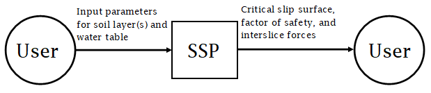
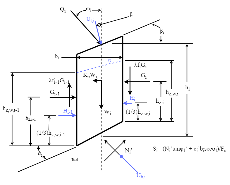
The mobilized shear force defined in GD:bsShrFEq can be substituted into the definition of mobilized shear force based on the factor of safety, from GD:mobShr yielding Equation (1) below:

\[\left({\symbf{W}}_{i}-{\symbf{X}}_{i-1}+{\symbf{X}}_{i}+{\symbf{U}_{\text{g},i}} \cos\left({\symbf{β}}_{i}\right)+{\symbf{Q}}_{i} \cos\left({\symbf{ω}}_{i}\right)\right) \sin\left({\symbf{α}}_{i}\right)-\left(-{K_{\text{c}}} {\symbf{W}}_{i}-{\symbf{G}}_{i}+{\symbf{G}}_{i-1}-{\symbf{H}}_{i}+{\symbf{H}}_{i-1}+{\symbf{U}_{\text{g},i}} \sin\left({\symbf{β}}_{i}\right)+{\symbf{Q}}_{i} \sin\left({\symbf{ω}}_{i}\right)\right) \cos\left({\symbf{α}}_{i}\right)=\frac{{\symbf{N'}}_{i} \tan\left(φ'\right)+c' {\symbf{L}_{b,i}}}{{F_{\text{S}}}}\]

An expression for the effective normal forces, N′, can be derived by substituting the normal forces equilibrium from GD:normForcEq into the definition for effective normal forces from GD:resShearWO. This results in Equation (2):

\[{\symbf{N'}}_{i}=\left({\symbf{W}}_{i}-{\symbf{X}}_{i-1}+{\symbf{X}}_{i}+{\symbf{U}_{\text{g},i}} \cos\left({\symbf{β}}_{i}\right)+{\symbf{Q}}_{i} \cos\left({\symbf{ω}}_{i}\right)\right) \cos\left({\symbf{α}}_{i}\right)+\left(-{K_{\text{c}}} {\symbf{W}}_{i}-{\symbf{G}}_{i}+{\symbf{G}}_{i-1}-{\symbf{H}}_{i}+{\symbf{H}}_{i-1}+{\symbf{U}_{\text{g},i}} \sin\left({\symbf{β}}_{i}\right)+{\symbf{Q}}_{i} \sin\left({\symbf{ω}}_{i}\right)\right) \sin\left({\symbf{α}}_{i}\right)-{\symbf{U}_{\text{b},i}}\]

Substituting Equation (2) into Equation (1) gives:

\[\left({\symbf{W}}_{i}-{\symbf{X}}_{i-1}+{\symbf{X}}_{i}+{\symbf{U}_{\text{g},i}} \cos\left({\symbf{β}}_{i}\right)+{\symbf{Q}}_{i} \cos\left({\symbf{ω}}_{i}\right)\right) \sin\left({\symbf{α}}_{i}\right)-\left(-{K_{\text{c}}} {\symbf{W}}_{i}-{\symbf{G}}_{i}+{\symbf{G}}_{i-1}-{\symbf{H}}_{i}+{\symbf{H}}_{i-1}+{\symbf{U}_{\text{g},i}} \sin\left({\symbf{β}}_{i}\right)+{\symbf{Q}}_{i} \sin\left({\symbf{ω}}_{i}\right)\right) \cos\left({\symbf{α}}_{i}\right)=\frac{\left(\left({\symbf{W}}_{i}-{\symbf{X}}_{i-1}+{\symbf{X}}_{i}+{\symbf{U}_{\text{g},i}} \cos\left({\symbf{β}}_{i}\right)+{\symbf{Q}}_{i} \cos\left({\symbf{ω}}_{i}\right)\right) \cos\left({\symbf{α}}_{i}\right)+\left(-{K_{\text{c}}} {\symbf{W}}_{i}-{\symbf{G}}_{i}+{\symbf{G}}_{i-1}-{\symbf{H}}_{i}+{\symbf{H}}_{i-1}+{\symbf{U}_{\text{g},i}} \sin\left({\symbf{β}}_{i}\right)+{\symbf{Q}}_{i} \sin\left({\symbf{ω}}_{i}\right)\right) \sin\left({\symbf{α}}_{i}\right)-{\symbf{U}_{\text{b},i}}\right) \tan\left(φ'\right)+c' {\symbf{L}_{b,i}}}{{F_{\text{S}}}}\]

Since the interslice shear forces X and interslice normal forces G are unknown, they are separated from the other terms as follows:

\[\left({\symbf{W}}_{i}+{\symbf{U}_{\text{g},i}} \cos\left({\symbf{β}}_{i}\right)+{\symbf{Q}}_{i} \cos\left({\symbf{ω}}_{i}\right)\right) \sin\left({\symbf{α}}_{i}\right)-\left(-{K_{\text{c}}} {\symbf{W}}_{i}-{\symbf{H}}_{i}+{\symbf{H}}_{i-1}+{\symbf{U}_{\text{g},i}} \sin\left({\symbf{β}}_{i}\right)+{\symbf{Q}}_{i} \sin\left({\symbf{ω}}_{i}\right)\right) \cos\left({\symbf{α}}_{i}\right)-\left(-{\symbf{G}}_{i}+{\symbf{G}}_{i-1}\right) \cos\left({\symbf{α}}_{i}\right)+\left(-{\symbf{X}}_{i-1}+{\symbf{X}}_{i}\right) \sin\left({\symbf{α}}_{i}\right)=\frac{\left(\left({\symbf{W}}_{i}+{\symbf{U}_{\text{g},i}} \cos\left({\symbf{β}}_{i}\right)+{\symbf{Q}}_{i} \cos\left({\symbf{ω}}_{i}\right)\right) \cos\left({\symbf{α}}_{i}\right)+\left(-{K_{\text{c}}} {\symbf{W}}_{i}-{\symbf{H}}_{i}+{\symbf{H}}_{i-1}+{\symbf{U}_{\text{g},i}} \sin\left({\symbf{β}}_{i}\right)+{\symbf{Q}}_{i} \sin\left({\symbf{ω}}_{i}\right)\right) \sin\left({\symbf{α}}_{i}\right)+\left(-{\symbf{G}}_{i}+{\symbf{G}}_{i-1}\right) \sin\left({\symbf{α}}_{i}\right)+\left(-{\symbf{X}}_{i-1}+{\symbf{X}}_{i}\right) \cos\left({\symbf{α}}_{i}\right)-{\symbf{U}_{\text{b},i}}\right) \tan\left(φ'\right)+c' {\symbf{L}_{b,i}}}{{F_{\text{S}}}}\]

Applying assumptions A:Seismic-Force and A:Surface-Load, which state that the seismic coefficient and the external forces, respectively, are zero, allows for further simplification as shown below:

\[\left({\symbf{W}}_{i}+{\symbf{U}_{\text{g},i}} \cos\left({\symbf{β}}_{i}\right)\right) \sin\left({\symbf{α}}_{i}\right)-\left(-{\symbf{H}}_{i}+{\symbf{H}}_{i-1}+{\symbf{U}_{\text{g},i}} \sin\left({\symbf{β}}_{i}\right)\right) \cos\left({\symbf{α}}_{i}\right)-\left(-{\symbf{G}}_{i}+{\symbf{G}}_{i-1}\right) \cos\left({\symbf{α}}_{i}\right)+\left(-{\symbf{X}}_{i-1}+{\symbf{X}}_{i}\right) \sin\left({\symbf{α}}_{i}\right)=\frac{\left(\left({\symbf{W}}_{i}+{\symbf{U}_{\text{g},i}} \cos\left({\symbf{β}}_{i}\right)\right) \cos\left({\symbf{α}}_{i}\right)+\left(-{\symbf{H}}_{i}+{\symbf{H}}_{i-1}+{\symbf{U}_{\text{g},i}} \sin\left({\symbf{β}}_{i}\right)\right) \sin\left({\symbf{α}}_{i}\right)+\left(-{\symbf{G}}_{i}+{\symbf{G}}_{i-1}\right) \sin\left({\symbf{α}}_{i}\right)+\left(-{\symbf{X}}_{i-1}+{\symbf{X}}_{i}\right) \cos\left({\symbf{α}}_{i}\right)-{\symbf{U}_{\text{b},i}}\right) \tan\left(φ'\right)+c' {\symbf{L}_{b,i}}}{{F_{\text{S}}}}\]

The definitions of GD:resShearWO and GD:mobShearWO are present in this equation, and thus can be replaced by R_i and T_i, respectively:

\[{\symbf{T}}_{i}+\left(-{\symbf{X}}_{i-1}+{\symbf{X}}_{i}\right) \sin\left({\symbf{α}}_{i}\right)-\left(-{\symbf{G}}_{i}+{\symbf{G}}_{i-1}\right) \cos\left({\symbf{α}}_{i}\right)=\frac{{\symbf{R}}_{i}+\left(\left(-{\symbf{X}}_{i-1}+{\symbf{X}}_{i}\right) \cos\left({\symbf{α}}_{i}\right)+\left(-{\symbf{G}}_{i}+{\symbf{G}}_{i-1}\right) \sin\left({\symbf{α}}_{i}\right)\right) \tan\left(φ'\right)}{{F_{\text{S}}}}\]

The interslice shear forces X can be expressed in terms of the interslice normal forces G using A:Interslice-Norm-Shear-Forces-Linear and GD:normShrR, resulting in:

\[{\symbf{T}}_{i}+\left(-λ {\symbf{f}}_{i-1} {\symbf{G}}_{i-1}+λ {\symbf{f}}_{i} {\symbf{G}}_{i}\right) \sin\left({\symbf{α}}_{i}\right)-\left(-{\symbf{G}}_{i}+{\symbf{G}}_{i-1}\right) \cos\left({\symbf{α}}_{i}\right)=\frac{{\symbf{R}}_{i}+\left(\left(-λ {\symbf{f}}_{i-1} {\symbf{G}}_{i-1}+λ {\symbf{f}}_{i} {\symbf{G}}_{i}\right) \cos\left({\symbf{α}}_{i}\right)+\left(-{\symbf{G}}_{i}+{\symbf{G}}_{i-1}\right) \sin\left({\symbf{α}}_{i}\right)\right) \tan\left(φ'\right)}{{F_{\text{S}}}}\]

Rearranging yields the following:

\[{\symbf{G}}_{i} \left(\left(λ {\symbf{f}}_{i} \cos\left({\symbf{α}}_{i}\right)-\sin\left({\symbf{α}}_{i}\right)\right) \tan\left(φ'\right)-\left(λ {\symbf{f}}_{i} \sin\left({\symbf{α}}_{i}\right)+\cos\left({\symbf{α}}_{i}\right)\right) {F_{\text{S}}}\right)={\symbf{G}}_{i-1} \left(\left(λ {\symbf{f}}_{i-1} \cos\left({\symbf{α}}_{i}\right)-\sin\left({\symbf{α}}_{i}\right)\right) \tan\left(φ'\right)-\left(λ {\symbf{f}}_{i-1} \sin\left({\symbf{α}}_{i}\right)+\cos\left({\symbf{α}}_{i}\right)\right) {F_{\text{S}}}\right)+{F_{\text{S}}} {\symbf{T}}_{i}-{\symbf{R}}_{i}\]

The definitions for Φ and Ψ from DD:convertFunc1 and DD:convertFunc2 simplify the above to Equation (3):

\[{\symbf{G}}_{i} {\symbf{Φ}}_{i}={\symbf{Ψ}}_{i-1} {\symbf{G}}_{i-1} {\symbf{Φ}}_{i-1}+{F_{\text{S}}} {\symbf{T}}_{i}-{\symbf{R}}_{i}\]

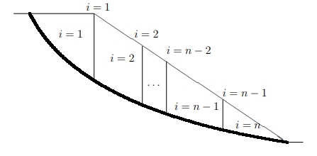
Versions of Equation (3) instantiated for slices 1 to n are shown below:

\[{\symbf{G}}_{1} {\symbf{Φ}}_{1}={\symbf{Ψ}}_{0} {\symbf{G}}_{0} {\symbf{Φ}}_{0}+{F_{\text{S}}} {\symbf{T}}_{1}-{\symbf{R}}_{1}\] \[{\symbf{G}}_{2} {\symbf{Φ}}_{2}={\symbf{Ψ}}_{1} {\symbf{G}}_{1} {\symbf{Φ}}_{1}+{F_{\text{S}}} {\symbf{T}}_{2}-{\symbf{R}}_{2}\] \[{\symbf{G}}_{3} {\symbf{Φ}}_{3}={\symbf{Ψ}}_{2} {\symbf{G}}_{2} {\symbf{Φ}}_{2}+{F_{\text{S}}} {\symbf{T}}_{3}-{\symbf{R}}_{3}\]

...

\[{\symbf{G}}_{n-2} {\symbf{Φ}}_{n-2}={\symbf{Ψ}}_{n-3} {\symbf{G}}_{n-3} {\symbf{Φ}}_{n-3}+{F_{\text{S}}} {\symbf{T}}_{n-2}-{\symbf{R}}_{n-2}\] \[{\symbf{G}}_{n-1} {\symbf{Φ}}_{n-1}={\symbf{Ψ}}_{n-2} {\symbf{G}}_{n-2} {\symbf{Φ}}_{n-2}+{F_{\text{S}}} {\symbf{T}}_{n-1}-{\symbf{R}}_{n-1}\] \[{\symbf{G}}_{n} {\symbf{Φ}}_{n}={\symbf{Ψ}}_{n-1} {\symbf{G}}_{n-1} {\symbf{Φ}}_{n-1}+{F_{\text{S}}} {\symbf{T}}_{n}-{\symbf{R}}_{n}\]

Applying A:Edge-Slices, which says that G₀ and G_n are zero, results in the following special cases: Equation (8) for the first slice:

\[{\symbf{G}}_{1} {\symbf{Φ}}_{1}={F_{\text{S}}} {\symbf{T}}_{1}-{\symbf{R}}_{1}\]

and Equation (9) for the nth slice:

\[-\left(\frac{{F_{\text{S}}} {\symbf{T}}_{n}-{\symbf{R}}_{n}}{{\symbf{Ψ}}_{n-1}}\right)={\symbf{G}}_{n-1} {\symbf{Φ}}_{n-1}\]

Substituting Equation (8) into Equation (4) yields Equation (10):

\[{\symbf{G}}_{2} {\symbf{Φ}}_{2}={\symbf{Ψ}}_{1} \left({F_{\text{S}}} {\symbf{T}}_{1}-{\symbf{R}}_{1}\right)+{F_{\text{S}}} {\symbf{T}}_{2}-{\symbf{R}}_{2}\]

which can be substituted into Equation (5) to get Equation (11):

\[{\symbf{G}}_{3} {\symbf{Φ}}_{3}={\symbf{Ψ}}_{2} \left({\symbf{Ψ}}_{1} \left({F_{\text{S}}} {\symbf{T}}_{1}-{\symbf{R}}_{1}\right)+{F_{\text{S}}} {\symbf{T}}_{2}-{\symbf{R}}_{2}\right)+{F_{\text{S}}} {\symbf{T}}_{3}-{\symbf{R}}_{3}\]

and so on until Equation (12) is obtained from Equation (7):

\[{\symbf{G}}_{n-1} {\symbf{Φ}}_{n-1}={\symbf{Ψ}}_{n-2} \left({\symbf{Ψ}}_{n-3} \left({\symbf{Ψ}}_{1} \left({F_{\text{S}}} {\symbf{T}}_{1}-{\symbf{R}}_{1}\right)+{F_{\text{S}}} {\symbf{T}}_{2}-{\symbf{R}}_{2}\right)+{F_{\text{S}}} {\symbf{T}}_{n-2}-{\symbf{R}}_{n-2}\right)+{F_{\text{S}}} {\symbf{T}}_{n-1}-{\symbf{R}}_{n-1}\]

Equation (9) can then be substituted into the left-hand side of Equation (12), resulting in:

\[-\left(\frac{{F_{\text{S}}} {\symbf{T}}_{n}-{\symbf{R}}_{n}}{{\symbf{Ψ}}_{n-1}}\right)={\symbf{Ψ}}_{n-2} \left({\symbf{Ψ}}_{n-3} \left({\symbf{Ψ}}_{1} \left({F_{\text{S}}} {\symbf{T}}_{1}-{\symbf{R}}_{1}\right)+{F_{\text{S}}} {\symbf{T}}_{2}-{\symbf{R}}_{2}\right)+{F_{\text{S}}} {\symbf{T}}_{n-2}-{\symbf{R}}_{n-2}\right)+{F_{\text{S}}} {\symbf{T}}_{n-1}-{\symbf{R}}_{n-1}\]

This can be rearranged by multiplying both sides by Ψ_n−1 and then distributing the multiplication of each Ψ over addition to obtain:

\[-\left({F_{\text{S}}} {\symbf{T}}_{n}-{\symbf{R}}_{n}\right)={\symbf{Ψ}}_{n-1} {\symbf{Ψ}}_{n-2} {\symbf{Ψ}}_{1} \left({F_{\text{S}}} {\symbf{T}}_{1}-{\symbf{R}}_{1}\right)+{\symbf{Ψ}}_{n-1} {\symbf{Ψ}}_{n-2} {\symbf{Ψ}}_{2} \left({F_{\text{S}}} {\symbf{T}}_{2}-{\symbf{R}}_{2}\right)+{\symbf{Ψ}}_{n-1} \left({F_{\text{S}}} {\symbf{T}}_{n-1}-{\symbf{R}}_{n-1}\right)\]

The multiplication of the Ψ terms can be further distributed over the subtractions, resulting in the equation having terms that each either contain an R or a T. The equation can then be rearranged so terms containing an R are on one side of the equality, and terms containing a T are on the other. The multiplication by the factor of safety is common to all of the T terms, and thus can be factored out, resulting in:

\[{F_{\text{S}}} \left({\symbf{Ψ}}_{n-1} {\symbf{Ψ}}_{n-2} {\symbf{Ψ}}_{1} {\symbf{T}}_{1}+{\symbf{Ψ}}_{n-1} {\symbf{Ψ}}_{n-2} {\symbf{Ψ}}_{2} {\symbf{T}}_{2}+{\symbf{Ψ}}_{n-1} {\symbf{T}}_{n-1}+{\symbf{T}}_{n}\right)={\symbf{Ψ}}_{n-1} {\symbf{Ψ}}_{n-2} {\symbf{Ψ}}_{1} {\symbf{R}}_{1}+{\symbf{Ψ}}_{n-1} {\symbf{Ψ}}_{n-2} {\symbf{Ψ}}_{2} {\symbf{R}}_{2}+{\symbf{Ψ}}_{n-1} {\symbf{R}}_{n-1}+{\symbf{R}}_{n}\]

Isolating the factor of safety on the left-hand side and using compact notation for the products and sums yields Equation (13), which can also be seen in IM:fctSfty:

\[{F_{\text{S}}}=\frac{\displaystyle\sum_{i=1}^{n-1}{{\symbf{R}}_{i} \displaystyle\prod_{v=i}^{n-1}{{\symbf{Ψ}}_{v}}}+{\symbf{R}}_{n}}{\displaystyle\sum_{i=1}^{n-1}{{\symbf{T}}_{i} \displaystyle\prod_{v=i}^{n-1}{{\symbf{Ψ}}_{v}}}+{\symbf{T}}_{n}}\]

F_S depends on the unknowns λ (IM:nrmShrFor) and G (IM:intsliceFs).

From the moment equilibrium of GD:momentEql with the primary assumption for the Morgenstern-Price method of A:Interslice-Norm-Shear-Forces-Linear and associated definition GD:normShrR, Equation (14) can be derived:

\[0=-{\symbf{G}}_{i} \left({\symbf{h}_{\text{z},i}}+\frac{{\symbf{b}}_{i}}{2} \tan\left({\symbf{α}}_{i}\right)\right)+{\symbf{G}}_{i-1} \left({\symbf{h}_{\text{z},i-1}}-\frac{{\symbf{b}}_{i}}{2} \tan\left({\symbf{α}}_{i}\right)\right)-{\symbf{H}}_{i} \left(\frac{1}{3} {\symbf{h}_{\text{z,w},i}}+\frac{{\symbf{b}}_{i}}{2} \tan\left({\symbf{α}}_{i}\right)\right)+{\symbf{H}}_{i-1} \left(\frac{1}{3} {\symbf{h}_{\text{z,w},i-1}}-\frac{{\symbf{b}}_{i}}{2} \tan\left({\symbf{α}}_{i}\right)\right)+λ \frac{{\symbf{b}}_{i}}{2} \left({\symbf{G}}_{i} {\symbf{f}}_{i}+{\symbf{G}}_{i-1} {\symbf{f}}_{i-1}\right)+\frac{-{K_{\text{c}}} {\symbf{W}}_{i} {\symbf{h}}_{i}}{2}+{\symbf{U}_{\text{g},i}} \sin\left({\symbf{β}}_{i}\right) {\symbf{h}}_{i}+{\symbf{Q}}_{i} \sin\left({\symbf{ω}}_{i}\right) {\symbf{h}}_{i}\]

Rearranging the equation in terms of λ leads to Equation (15):

\[λ=\frac{-{\symbf{G}}_{i} \left({\symbf{h}_{\text{z},i}}+\frac{{\symbf{b}}_{i}}{2} \tan\left({\symbf{α}}_{i}\right)\right)+{\symbf{G}}_{i-1} \left({\symbf{h}_{\text{z},i-1}}-\frac{{\symbf{b}}_{i}}{2} \tan\left({\symbf{α}}_{i}\right)\right)-{\symbf{H}}_{i} \left(\frac{1}{3} {\symbf{h}_{\text{z,w},i}}+\frac{{\symbf{b}}_{i}}{2} \tan\left({\symbf{α}}_{i}\right)\right)+{\symbf{H}}_{i-1} \left(\frac{1}{3} {\symbf{h}_{\text{z,w},i-1}}-\frac{{\symbf{b}}_{i}}{2} \tan\left({\symbf{α}}_{i}\right)\right)+\frac{-{K_{\text{c}}} {\symbf{W}}_{i} {\symbf{h}}_{i}}{2}+{\symbf{U}_{\text{g},i}} \sin\left({\symbf{β}}_{i}\right) {\symbf{h}}_{i}+{\symbf{Q}}_{i} \sin\left({\symbf{ω}}_{i}\right) {\symbf{h}}_{i}}{-\frac{{\symbf{b}}_{i}}{2} \left({\symbf{G}}_{i} {\symbf{f}}_{i}+{\symbf{G}}_{i-1} {\symbf{f}}_{i-1}\right)}\]

This equation can be simplified by applying assumptions A:Seismic-Force and A:Surface-Load, which state that the seismic and external forces, respectively, are zero:

\[λ=\frac{-{\symbf{G}}_{i} \left({\symbf{h}_{\text{z},i}}+\frac{{\symbf{b}}_{i}}{2} \tan\left({\symbf{α}}_{i}\right)\right)+{\symbf{G}}_{i-1} \left({\symbf{h}_{\text{z},i-1}}-\frac{{\symbf{b}}_{i}}{2} \tan\left({\symbf{α}}_{i}\right)\right)-{\symbf{H}}_{i} \left(\frac{1}{3} {\symbf{h}_{\text{z,w},i}}+\frac{{\symbf{b}}_{i}}{2} \tan\left({\symbf{α}}_{i}\right)\right)+{\symbf{H}}_{i-1} \left(\frac{1}{3} {\symbf{h}_{\text{z,w},i-1}}-\frac{{\symbf{b}}_{i}}{2} \tan\left({\symbf{α}}_{i}\right)\right)+{\symbf{U}_{\text{g},i}} \sin\left({\symbf{β}}_{i}\right) {\symbf{h}}_{i}}{-\frac{{\symbf{b}}_{i}}{2} \left({\symbf{G}}_{i} {\symbf{f}}_{i}+{\symbf{G}}_{i-1} {\symbf{f}}_{i-1}\right)}\]

Taking the summation of all slices, and applying A:Edge-Slices to set G₀, G_n, H₀, and H_n equal to zero, a general equation for the proportionality constant λ is developed in Equation (16), which combines IM:nrmShrFor, IM:nrmShrForNum, and IM:nrmShrForDen:

\[λ=\frac{\displaystyle\sum_{i=1}^{n}{{\symbf{b}}_{i} \left({{\symbf{F}_{\text{x}}}^{\text{G}}}+{{\symbf{F}_{\text{x}}}^{\text{H}}}\right) \tan\left({\symbf{α}}_{i}\right)+{\symbf{h}}_{i} -2 {\symbf{U}_{\text{g},i}} \sin\left({\symbf{β}}_{i}\right)}}{\displaystyle\sum_{i=1}^{n}{{\symbf{b}}_{i} \left({\symbf{G}}_{i} {\symbf{f}}_{i}+{\symbf{G}}_{i-1} {\symbf{f}}_{i-1}\right)}}\]

Equation (16) for λ is a function of the unknown interslice normal forces G (IM:intsliceFs) which itself depends on the unknown factor of safety F_S (IM:fctSfty).

See IM:nrmShrFor for the derivation of C_num.

See IM:nrmShrFor for the derivation of C_den.

This derivation is identical to the derivation for IM:fctSfty up until Equation (3) shown again below:

\[{\symbf{G}}_{i} {\symbf{Φ}}_{i}={\symbf{Ψ}}_{i-1} {\symbf{G}}_{i-1} {\symbf{Φ}}_{i-1}+{F_{\text{S}}} {\symbf{T}}_{i}-{\symbf{R}}_{i}\]

A simple rearrangement of Equation (3) leads to Equation (17), also seen in IM:intsliceFs:

\[{\symbf{G}}_{i}=\frac{{\symbf{Ψ}}_{i-1} {\symbf{G}}_{i-1}+{F_{\text{S}}} {\symbf{T}}_{i}-{\symbf{R}}_{i}}{{\symbf{Φ}}_{i}}\]

The cases shown in IM:intsliceFs for when i = 0, i = 1, or i = n are derived by applying A:Edge-Slices, which says that G₀ and G_n are zero, to Equation (17). G depends on the unknowns F_S (IM:fctSfty) and λ (IM:nrmShrFor).