Table of Contents

An outline of all sections included in this SRS is recorded here for easy reference.

• Table of Contents
• Reference Material
  • Table of Units
  • Table of Symbols
  • Abbreviations and Acronyms
• Introduction
  • Purpose of Document
  • Scope of Requirements
  • Characteristics of Intended Reader
  • Organization of Document
• General System Description
  • System Context
  • User Characteristics
  • System Constraints
• Specific System Description
  • Problem Description
    • Terminology and Definitions
    • Physical System Description
    • Goal Statements
  • Solution Characteristics Specification
    • Assumptions
    • Theoretical Models
    • General Definitions
    • Data Definitions
    • Instance Models
    • Data Constraints
• Requirements
  • Functional Requirements
  • Non-Functional Requirements
• Likely Changes
• Traceability Matrices and Graphs
• References

Reference Material

This section records information for easy reference.

Introduction

Automatic process control with a controller (P/PI/PD/PID) is used in a variety of applications such as thermostats, automobile cruise-control, etc. The gains of a controller in an application must be tuned before the controller is ready for production. Therefore a simulation of the PD Controller with a Second Order System is created in this project that can be used to tune the gain constants.

The following section provides an overview of the Software Requirements Specification (SRS) for PD Controller. This section explains the purpose of this document, the scope of the requirements, the characteristics of the intended reader, and the organization of the document.

General System Description

This section provides general information about the system. It identifies the interfaces between the system and its environment, describes the user characteristics, and lists the system constraints.

System Context

Fig:systemContextDiag shows the system context. The circle represents an external entity outside the software, the user in this case. The rectangle represents the software system itself, PD Controller in this case. Arrows are used to show the data flow between the system and its environment.

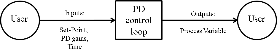
PD Controller is self-contained. The only external interaction is with the user. The responsibilities of the user and the system are as follows:

• User Responsibilities
  • Feed inputs to the model
  • Review the response of the Power Plant
  • Tune the controller gains
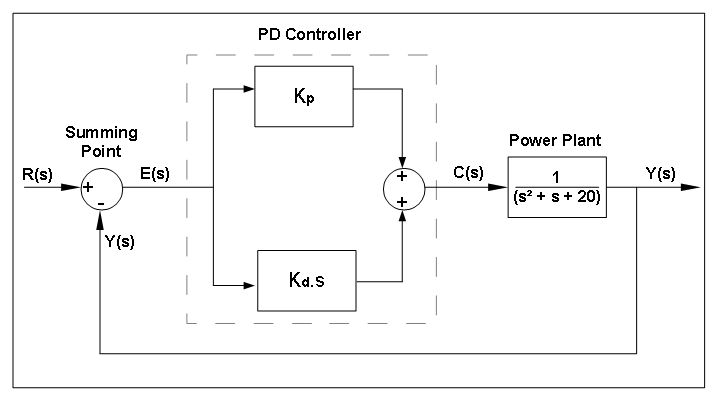
• PD Controller Responsibilities
  • Check the validity of the inputs
  • Calculate the outputs of the PD Controller and Power Plant

Specific System Description

This section first presents the problem description, which gives a high-level view of the problem to be solved. This is followed by the solution characteristics specification, which presents the assumptions, theories, and definitions that are used.

Problem Description

A system is needed to provide a model of a PD Controller that can be used for the tuning of the gain constants before the deployment of the controller.

Terminology and Definitions

This subsection provides a list of terms that are used in the subsequent sections and their meaning, with the purpose of reducing ambiguity and making it easier to correctly understand the requirements.

• PD Control Loop: Closed-Loop control system with PD Controller, Summing Point and Power Plant.
• PD Controller: Proportional-Derivative Controller.
• Summing Point: Control block where the difference between the Set-Point and the Process Variable is computed.
• Power Plant: A second order system to be controlled.
• Second Order System: A system whose input-output relationship is denoted by a second-order differential equation.
• Process Error: Input to the PID controller. Process Error is the difference between the Set-Point and the Process Variable.
• Simulation Time: Total execution time of the PD simulation.
• Process Variable: The output value from the power plant.
• Set-Point: The desired value that the control system must reach. This also knows as the reference variable.
• Proportional Gain: Gain constant of the proportional controller.
• Derivative Gain: Gain constant of the derivative controller.
• Proportional control: A linear feedback control system where correction is applied to the controlled variable which is proportional to the difference between desired and measured values.
• Derivative control: Monitors the rate of change of the error signal and contributes a component of the output signal (proportional to a derivative of the error signal).
• Frequency domain: The analysis of mathematical functions in terms of frequency, instead of time.
• Time domain: The analysis of mathematical functions in terms of time.
• Laplace transform: An integral transform that converts a function of a real variable t (often time) to a function of a complex variable s (complex frequency).
• Control Variable: The Control Variable is the output of the PD controller.
• Step Time: Simulation step time.
• Absolute Tolerance: Absolute tolerance for the integrator.
• Relative Tolerance: Relative tolerance for the integrator.
• Transfer Function: The Transfer Function of a system is the ratio of the output to the input functions in the frequency domain.
• Damping Coefficient: Quantity that characterizes a second order system's oscillatory response.
• Stiffness Coefficient: Quantity that characterizes a spring's stiffness.

Physical System Description

The physical system of PD Controller, as shown in Fig:pidSysDiagram, includes the following elements:

PS1: The Summing Point.

PS2: The PD Controller.

PS3: The Power Plant.

Goal Statements

Given Set-Point, Simulation Time, Proportional Gain, Derivative Gain, and Step Time, the goal statement is:

Process-Variable: Calculate the output of the Power Plant (Process Variable) over time.

Requirements

This section provides the functional requirements, the tasks and behaviours that the software is expected to complete, and the non-functional requirements, the qualities that the software is expected to exhibit.

Likely Changes

This section lists the likely changes to be made to the software.

Traceability Matrices and Graphs

The purpose of the traceability matrices is to provide easy references on what has to be additionally modified if a certain component is changed. Every time a component is changed, the items in the column of that component that are marked with an "X" should be modified as well. Tab:TraceMatAvsA shows the dependencies of the assumptions on each other. Tab:TraceMatAvsAll shows the dependencies of the data definitions, theoretical models, general definitions, instance models, requirements, likely changes, and unlikely changes on the assumptions. Tab:TraceMatRefvsRef shows the dependencies of the data definitions, theoretical models, general definitions, and instance models on each other. Tab:TraceMatAllvsR shows the dependencies of the requirements and goal statements on the data definitions, theoretical models, general definitions, and instance models.

The purpose of the traceability graphs is also to provide easy references on what has to be additionally modified if a certain component is changed. The arrows in the graphs represent dependencies. The component at the tail of an arrow is depended on by the component at the head of that arrow. Therefore, if a component is changed, the components that it points to should also be changed. Fig:TraceGraphAvsA shows the dependencies of assumptions on each other. Fig:TraceGraphAvsAll shows the dependencies of data definitions, theoretical models, general definitions, instance models, requirements, likely changes, and unlikely changes on the assumptions. Fig:TraceGraphRefvsRef shows the dependencies of data definitions, theoretical models, general definitions, and instance models on each other. Fig:TraceGraphAllvsR shows the dependencies of requirements and goal statements on the data definitions, theoretical models, general definitions, and instance models. Fig:TraceGraphAllvsAll shows the dependencies of dependencies of assumptions, models, definitions, requirements, goals, and changes with each other.

For convenience, the following graphs can be found at the links below:

• TraceGraphAvsA
• TraceGraphAvsAll
• TraceGraphRefvsRef
• TraceGraphAllvsR
• TraceGraphAllvsAll

References

• [1]: Abbasi, Nasser M. A differential equation view of closed loop control systems. November, 2020. https://www.12000.org/my_notes/connecting_systems/report.htm.
• [2]: Johnson, Michael A. and Moradi, Mohammad H. PID Control: New Identification and Design Methods, Chapter 1. Springer Science and Business Media, 2006. Print.
• [3]: Koothoor, Nirmitha. A Document Driven Approach to Certifying Scientific Computing Software. McMaster University, Hamilton, ON, Canada: 2013. Print.
• [4]: Smith, W. Spencer and Koothoor, Nirmitha. "A Document-Driven Method for Certifying Scientific Computing Software for Use in Nuclear Safety Analysis." Nuclear Engineering and Technology, vol. 48, no. 2, April, 2016. http://www.sciencedirect.com/science/article/pii/S1738573315002582. pp. 404–418.
• [5]: Smith, W. Spencer and Lai, Lei. "A new requirements template for scientific computing." Proceedings of the First International Workshop on Situational Requirements Engineering Processes - Methods, Techniques and Tools to Support Situation-Specific Requirements Engineering Processes, SREP'05. Edited by PJ Agerfalk, N. Kraiem, and J. Ralyte, Paris, France: 2005. pp. 107–121. In conjunction with 13th IEEE International Requirements Engineering Conference,
• [6]: Smith, W. Spencer, Lai, Lei, and Khedri, Ridha. "Requirements Analysis for Engineering Computation: A Systematic Approach for Improving Software Reliability." Reliable Computing, Special Issue on Reliable Engineering Computation, vol. 13, no. 1, February, 2007. https://doi.org/10.1007/s11155-006-9020-7. pp. 83–107.
• [7]: Wikipedia Contributors. Laplace transform. November, 2020. https://en.wikipedia.org/wiki/Laplace_transform.
• [8]: Wikipedia Contributors. PID controller. October, 2020. https://en.wikipedia.org/wiki/PID_controller.