Software Requirements Specification for GamePhysics

Alex Halliwushka, Luthfi Mawarid, and Olu Owojaiye

Table of Contents

An outline of all sections included in this SRS is recorded here for easy reference.

Reference Material

This section records information for easy reference.

Table of Units

The unit system used throughout is SI (Système International d'Unités). In addition to the basic units, several derived units are also used. For each unit, the Table of Units lists the symbol, a description, and the SI name.

Symbol Description SI Name
J energy joule
kg mass kilogram
m length metre
N force newton
rad angle radian
s time second

Table of Units

Table of Symbols

The symbols used in this document are summarized in the Table of Symbols along with their units. Throughout the document, symbols in bold will represent vectors, and scalars otherwise. The symbols are listed in alphabetical order. For vector quantities, the units shown are for each component of the vector.

Symbol Description Units
a(t) Linear acceleration \(\frac{\text{m}}{\text{s}^{2}}\)
a(t) Acceleration \(\frac{\text{m}}{\text{s}^{2}}\)
a(t)j J-Th Body's Acceleration \(\frac{\text{m}}{\text{s}^{2}}\)
CR Coefficient of restitution --
dj Distance Between the J-Th Particle and the Axis of Rotation m
d Distance between the center of mass of the rigid bodies m
Unit vector directed from the center of the large mass to the center of the smaller mass m
||d|| Euclidean norm of the distance between the center of mass of two bodies m
||d||2 Squared distance m2
F Force N
F1 Force exerted by the first body (on another body) N
F2 Force exerted by the second body (on another body) N
Fg Force of gravity N
Fj Force Applied to the J-Th Body at Time T N
G Gravitational constant \(\frac{\text{m}^{3}}{\text{kg}\text{s}^{2}}\)
g Gravitational acceleration \(\frac{\text{m}}{\text{s}^{2}}\)
h Height m
I Moment of inertia kgm2
IA Moment of Inertia of Rigid Body A kgm2
IB Moment of Inertia of Rigid Body B kgm2
J Impulse (vector) Ns
j Impulse (scalar) Ns
KE Kinetic energy J
L Length m
M Mass of the Larger Rigid Body kg
m Mass kg
m1 Mass of the first body kg
m2 Mass of the second body kg
mA Mass of Rigid Body A kg
mB Mass of Rigid Body B kg
mj Mass of the J-Th Particle kg
mT Total Mass of the Rigid Body kg
n Collision normal vector m
||n|| Length of the normal vector m
PE Potential energy J
p(t) Position m
p(t)CM Center of Mass m
p(t)j Position Vector of the J-Th Particle m
r Position vector m
t Time s
tc Denotes the time at collision s
u(t) Linear displacement m
u Displacement m
||uAP*n|| Length of the Perpendicular Vector to the Contact Displacement Vector of Rigid Body A m
||uBP*n|| Length of the Perpendicular Vector to the Contact Displacement Vector of Rigid Body B m
uOB Displacement vector between the origin and point B m
v(t) Linear velocity \(\frac{\text{m}}{\text{s}}\)
v(t) Velocity \(\frac{\text{m}}{\text{s}}\)
Δv Change in velocity \(\frac{\text{m}}{\text{s}}\)
v(t)AP Velocity of the Point of Collision P in Body A \(\frac{\text{m}}{\text{s}}\)
v(t)BP Velocity of the Point of Collision P in Body B \(\frac{\text{m}}{\text{s}}\)
v(t)1 Velocity of the First Body \(\frac{\text{m}}{\text{s}}\)
v(t)2 Velocity of the Second Body \(\frac{\text{m}}{\text{s}}\)
v(t)A Velocity at Point A \(\frac{\text{m}}{\text{s}}\)
v(t)B Velocity at Point B \(\frac{\text{m}}{\text{s}}\)
v(t)fAB Final Relative Velocity Between Rigid Bodies of A and B \(\frac{\text{m}}{\text{s}}\)
v(t)iAB Initial Relative Velocity Between Rigid Bodies of A and B \(\frac{\text{m}}{\text{s}}\)
v(t)j Velocity of the J-Th Body \(\frac{\text{m}}{\text{s}}\)
v(t)O Velocity at Point Origin \(\frac{\text{m}}{\text{s}}\)
α Angular acceleration \(\frac{\text{rad}}{\text{s}^{2}}\)
αj J-Th Body's Angular Acceleration \(\frac{\text{rad}}{\text{s}^{2}}\)
θ Angular displacement rad
τ Torque Nm
τj Torque applied to the j-th body Nm
ω Angular velocity \(\frac{\text{rad}}{\text{s}}\)
ϕ Orientation rad

Table of Symbols

Abbreviations and Acronyms

Abbreviation Full Form
2D Two-Dimensional
3D Three-Dimensional
A Assumption
CM Centre of Mass
DD Data Definition
GD General Definition
GS Goal Statement
IM Instance Model
LC Likely Change
ODE Ordinary Differential Equation
R Requirement
RefBy Referenced by
Refname Reference Name
SRS Software Requirements Specification
TM Theoretical Model
UC Unlikely Change
Uncert. Typical Uncertainty

Abbreviations and Acronyms

Introduction

Due to the rising cost of developing video games, developers are looking for ways to save time and money for their projects. Using an open source physics library that is reliable and free will cut down development costs and lead to better quality products.

The following section provides an overview of the Software Requirements Specification (SRS) for GamePhysics. This section explains the purpose of this document, the scope of the requirements, the characteristics of the intended reader, and the organization of the document.

Purpose of Document

The primary purpose of this document is to record the requirements of GamePhysics. Goals, assumptions, theoretical models, definitions, and other model derivation information are specified, allowing the reader to fully understand and verify the purpose and scientific basis of GamePhysics. With the exception of system constraints, this SRS will remain abstract, describing what problem is being solved, but not how to solve it.

This document will be used as a starting point for subsequent development phases, including writing the design specification and the software verification and validation plan. The design document will show how the requirements are to be realized, including decisions on the numerical algorithms and programming environment. The verification and validation plan will show the steps that will be used to increase confidence in the software documentation and the implementation. Although the SRS fits in a series of documents that follow the so-called waterfall model, the actual development process is not constrained in any way. Even when the waterfall model is not followed, as Parnas and Clements point out parnasClements1986, the most logical way to present the documentation is still to "fake" a rational design process.

Scope of Requirements

The scope of the requirements includes the physical simulation of 2D rigid bodies acted on by forces.

Characteristics of Intended Reader

Reviewers of this documentation should have an understanding of rigid body dynamics and high school calculus. The users of GamePhysics can have a lower level of expertise, as explained in Sec:User Characteristics.

Organization of Document

The organization of this document follows the template for an SRS for scientific computing software proposed by koothoor2013, smithLai2005, smithEtAl2007, and smithKoothoor2016. The presentation follows the standard pattern of presenting goals, theories, definitions, and assumptions. For readers that would like a more bottom up approach, they can start reading the instance models and trace back to find any additional information they require.

The goal statements are refined to the theoretical models and the theoretical models to the instance models.

General System Description

This section provides general information about the system. It identifies the interfaces between the system and its environment, describes the user characteristics, and lists the system constraints.

System Context

Fig:sysCtxDiag shows the system context. A circle represents an entity external to the software, the user in this case. A rectangle represents the software system itself (GamePhysics). Arrows are used to show the data flow between the system and its environment.

System Context
System Context

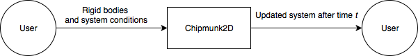
The interaction between the product and the user is through an application programming interface. The responsibilities of the user and the system are as follows:

  • User Responsibilities
    • Provide initial conditions of the physical state of the simulation, rigid bodies present, and forces applied to them.
    • Ensure application programming interface use complies with the user guide.
    • Ensure required software assumptions are appropriate for any particular problem the software addresses.
  • GamePhysics Responsibilities
    • Determine if the inputs and simulation state satisfy the required physical and system constraints.
    • Calculate the new state of all rigid bodies within the simulation at each simulation step.
    • Provide updated physical state of all rigid bodies at the end of a simulation step.

User Characteristics

The end user of GamePhysics should have an understanding of first year programming concepts and an understanding of high school physics.

System Constraints

There are no system constraints.

Specific System Description

This section first presents the problem description, which gives a high-level view of the problem to be solved. This is followed by the solution characteristics specification, which presents the assumptions, theories, and definitions that are used.

Problem Description

A system is needed to simulate 2D rigid body physics for use in game development in a simple, lightweight, fast, and portable manner, which will allow for the production of higher quality products. Creating a gaming physics library is a difficult task. Games need physics libraries that simulate objects acting under various physical conditions, while simultaneously being fast and efficient enough to work in soft real-time during the game. Developing a physics library from scratch takes a long period of time and is very costly, presenting barriers of entry which make it difficult for game developers to include physics in their products. There are a few free, open source and high quality physics libraries available to be used for consumer products.

Terminology and Definitions

This subsection provides a list of terms that are used in the subsequent sections and their meaning, with the purpose of reducing ambiguity and making it easier to correctly understand the requirements.

  • Rigid body: A solid body in which deformation is neglected.
  • Elasticity: The ratio of the relative velocities of two colliding objects after and before a collision.
  • Centre of mass: The mean location of the distribution of mass of the object.
  • Cartesian coordinate system: A coordinate system that specifies each point uniquely in a plane by a set of numerical coordinates, which are the signed distances to the point from two fixed perpendicular oriented lines, measured in the same unit of length (from cartesianWiki).
  • Right-handed coordinate system: A coordinate system where the positive z-axis comes out of the screen..
  • line: An interval between two points (from lineSource).
  • point: An exact location, it has no size, only position (from pointSource).
  • damping: An influence within or upon an oscillatory system that has the effect of reducing, restricting or preventing its oscillations (from dampingSource).

Goal Statements

Given the kinematic properties, and forces (including any collision forces) applied on a set of rigid bodies, the goal statements are:

Determine-Linear-Properties: Determine their new positions and velocities over a period of time.

Determine-Angular-Properties: Determine their new orientations and angular velocities over a period of time.

Solution Characteristics Specification

The instance models that govern GamePhysics are presented in the Instance Model Section. The information to understand the meaning of the instance models and their derivation is also presented, so that the instance models can be verified.

Assumptions

This section simplifies the original problem and helps in developing the theoretical models by filling in the missing information for the physical system. The assumptions refine the scope by providing more detail.

coordinateSystemTy: The library uses a Cartesian coordinate system.

axesDefined: The axes are defined using right-handed coordinate system. (RefBy: GD:impulse, IM:rotMot, and IM:col2D.)

collisionType: All rigid bodies collisions are vertex-to-edge collisions. (RefBy: GD:impulse, LC:Expanded-Collisions, and IM:col2D.)

dampingInvolvement: There is no damping involved throughout the simulation and this implies that there are no friction forces. (RefBy: IM:transMot, DD:potEnergy, LC:Include-Dampening, DD:kEnergy, and IM:col2D.)

constraintsAndJointsInvolvement: There are no constraints and joints involved throughout the simulation. (RefBy: IM:transMot, LC:Include-Joints-Constraints, and IM:col2D.)

Theoretical Models

This section focuses on the general equations and laws that GamePhysics is based on.

Refname TM:NewtonSecLawMot
Label

Newton's second law of motion

Equation \[\symbf{F}=m \symbf{a}\text{(}t\text{)}\]
Description
  • F is the force (N)
  • m is the mass (kg)
  • a(t) is the acceleration (\(\frac{\text{m}}{\text{s}^{2}}\))
Notes

The net force F on a body is proportional to the acceleration a(t) of the body, where m denotes the mass of the body as the constant of proportionality.

Source

--

RefBy

IM:transMot

Refname TM:NewtonThirdLawMot
Label

Newton's third law of motion

Equation \[{\symbf{F}_{1}}=-{\symbf{F}_{2}}\]
Description
  • F1 is the force exerted by the first body (on another body) (N)
  • F2 is the force exerted by the second body (on another body) (N)
Notes

Every action has an equal and opposite reaction. In other words, the force F1 exerted on the second rigid body by the first is equal in magnitude and in the opposite direction to the force F2 exerted on the first rigid body by the second.

Source

--

RefBy

Refname TM:UniversalGravLaw
Label

Newton's law of universal gravitation

Equation \[\symbf{F}=G \frac{{m_{1}} {m_{2}}}{\|\symbf{d}\|^{2}} \symbf{\hat{d}}=G \frac{{m_{1}} {m_{2}}}{\|\symbf{d}\|^{2}} \frac{\symbf{d}}{\|\symbf{d}\|}\]
Description
  • F is the force (N)
  • G is the gravitational constant (\(\frac{\text{m}^{3}}{\text{kg}\text{s}^{2}}\))
  • m1 is the mass of the first body (kg)
  • m2 is the mass of the second body (kg)
  • ||d|| is the Euclidean norm of the distance between the center of mass of two bodies (m)
  • is the unit vector directed from the center of the large mass to the center of the smaller mass (m)
  • d is the distance between the center of mass of the rigid bodies (m)
Notes

Two rigid bodies in the universe attract each other with a force F that is directly proportional to the product of their masses, m1 and m2, and inversely proportional to the squared distance ||d||2 between them.

Source

--

RefBy

GD:accelGravity

Refname TM:NewtonSecLawRotMot
Label

Newton's second law for rotational motion

Equation \[\symbf{τ}=\symbf{I} α\]
Description
  • τ is the torque (Nm)
  • I is the moment of inertia (kgm2)
  • α is the angular acceleration (\(\frac{\text{rad}}{\text{s}^{2}}\))
Notes

The net torque τ on a rigid body is proportional to its angular acceleration α, where I denotes the moment of inertia of the rigid body as the constant of proportionality.

We also assume that all rigid bodies involved are two-dimensional (from A:objectDimension).

Source

--

RefBy

IM:rotMot

General Definitions

This section collects the laws and equations that will be used to build the instance models.

Refname GD:accelGravity
Label

Acceleration due to gravity

Units

\(\frac{\text{m}}{\text{s}^{2}}\)

Equation \[\symbf{g}=-\frac{G M}{\|\symbf{d}\|^{2}} \symbf{\hat{d}}\]
Description
  • g is the gravitational acceleration (\(\frac{\text{m}}{\text{s}^{2}}\))
  • G is the gravitational constant (\(\frac{\text{m}^{3}}{\text{kg}\text{s}^{2}}\))
  • M is the mass of the larger rigid body (kg)
  • ||d|| is the Euclidean norm of the distance between the center of mass of two bodies (m)
  • is the unit vector directed from the center of the large mass to the center of the smaller mass (m)
Notes

If one of the masses is much larger than the other, it is convenient to define a gravitational field around the larger mass as shown above. The negative sign in the equation indicates that the force is an attractive force.

Source

Definition of Gravitational Acceleration

RefBy

IM:transMot

Detailed derivation of gravitational acceleration:

From Newton's law of universal gravitation, we have:

\[\symbf{F}=\frac{G {m_{1}} {m_{2}}}{{\|\symbf{d}\|^{2}}} \symbf{\hat{d}}\]

The above equation governs the gravitational attraction between two bodies. Suppose that one of the bodies is significantly more massive than the other, so that we concern ourselves with the force the massive body exerts on the lighter body. Further, suppose that the Cartesian coordinate system is chosen such that this force acts on a line which lies along one of the principal axes. Then our unit vector directed from the center of the large mass to the center of the smaller mass for the x or y axes is:

\[\symbf{\hat{d}}=\frac{\symbf{d}}{\|\symbf{d}\|}\]

Given the above assumptions, let M and m be the mass of the massive and light body respectively. Equating F above with Newton's second law for the force experienced by the light body, we get:

\[{\symbf{F}_{\symbf{g}}}=G \frac{M m}{{\|\symbf{d}\|^{2}}} \symbf{\hat{d}}=m \symbf{g}\]

where g is the gravitational acceleration. Dividing the above equation by m, we have:

\[G \frac{M}{{\|\symbf{d}\|^{2}}} \symbf{\hat{d}}=\symbf{g}\]

and thus the negative sign indicates that the force is an attractive force:

\[\symbf{g}=-G \frac{M}{{\|\symbf{d}\|^{2}}} \symbf{\hat{d}}\]
Refname GD:impulse
Label

Impulse for Collision

Units

Ns

Equation \[j=\frac{-\left(1+{C_{\text{R}}}\right) {{\symbf{v}\text{(}t\text{)}_{\text{i}}}^{\text{A}\text{B}}}\cdot{}\symbf{n}}{\left(\frac{1}{{m_{\text{A}}}}+\frac{1}{{m_{\text{B}}}}\right) \|\symbf{n}\|^{2}+\frac{\|{\symbf{u}_{\text{A}\text{P}}}\text{*}\symbf{n}\|^{2}}{{\symbf{I}_{\text{A}}}}+\frac{\|{\symbf{u}_{\text{B}\text{P}}}\text{*}\symbf{n}\|^{2}}{{\symbf{I}_{\text{B}}}}}\]
Description
  • j is the impulse (scalar) (Ns)
  • CR is the coefficient of restitution (Unitless)
  • v(t)iAB is the initial relative velocity between rigid bodies of A and B (\(\frac{\text{m}}{\text{s}}\))
  • n is the collision normal vector (m)
  • mA is the mass of rigid body A (kg)
  • mB is the mass of rigid body B (kg)
  • ||n|| is the length of the normal vector (m)
  • ||uAP*n|| is the length of the perpendicular vector to the contact displacement vector of rigid body A (m)
  • IA is the moment of inertia of rigid body A (kgm2)
  • ||uBP*n|| is the length of the perpendicular vector to the contact displacement vector of rigid body B (m)
  • IB is the moment of inertia of rigid body B (kgm2)
Notes

All bodies are assumed to be rigid (from A:objectTy) and two-dimensional (from A:objectDimension).

A right-handed coordinate system is used (from A:axesDefined).

All collisions are vertex-to-edge (from A:collisionType).

Source

Impulse for Collision Ref

RefBy

IM:col2D

Data Definitions

This section collects and defines all the data needed to build the instance models.

Refname DD:ctrOfMass
Label

Center of Mass

Symbol

p(t)CM

Units

m

Equation \[{\symbf{p}\text{(}t\text{)}_{\text{CM}}}=\frac{\displaystyle\sum{{m_{j}} {\symbf{p}\text{(}t\text{)}_{j}}}}{{m_{T}}}\]
Description
  • p(t)CM is the Center of Mass (m)
  • mj is the mass of the j-th particle (kg)
  • p(t)j is the position vector of the j-th particle (m)
  • mT is the total mass of the rigid body (kg)
Notes

All bodies are assumed to be rigid (from A:objectTy).

Source

--

RefBy

IM:transMot and IM:col2D

Refname DD:linDisp
Label

Linear displacement

Symbol

u(t)

Units

m

Equation \[u\text{(}t\text{)}=\frac{\,d\symbf{p}\text{(}t\text{)}\left(t\right)}{\,dt}\]
Description
  • u(t) is the linear displacement (m)
  • t is the time (s)
  • p(t) is the position (m)
Notes

All bodies are assumed to be rigid (from A:objectTy).

Source

--

RefBy

IM:transMot

Refname DD:linVel
Label

Linear velocity

Symbol

v(t)

Units

\(\frac{\text{m}}{\text{s}}\)

Equation \[v\text{(}t\text{)}=\frac{\,d\symbf{u}\left(t\right)}{\,dt}\]
Description
  • v(t) is the linear velocity (\(\frac{\text{m}}{\text{s}}\))
  • t is the time (s)
  • u is the displacement (m)
Notes

All bodies are assumed to be rigid (from A:objectTy).

Source

--

RefBy

IM:transMot

Refname DD:linAcc
Label

Linear acceleration

Symbol

a(t)

Units

\(\frac{\text{m}}{\text{s}^{2}}\)

Equation \[a\text{(}t\text{)}=\frac{\,d\symbf{v}\text{(}t\text{)}\left(t\right)}{\,dt}\]
Description
  • a(t) is the linear acceleration (\(\frac{\text{m}}{\text{s}^{2}}\))
  • t is the time (s)
  • v(t) is the velocity (\(\frac{\text{m}}{\text{s}}\))
Notes

All bodies are assumed to be rigid (from A:objectTy).

Source

--

RefBy

IM:transMot

Refname DD:angDisp
Label

Angular displacement

Symbol

θ

Units

rad

Equation \[θ=\frac{\,dϕ\left(t\right)}{\,dt}\]
Description
  • θ is the angular displacement (rad)
  • t is the time (s)
  • ϕ is the orientation (rad)
Notes

All bodies are assumed to be rigid (from A:objectTy) and two-dimensional (from A:objectDimension).

Source

--

RefBy

IM:rotMot

Refname DD:angVel
Label

Angular velocity

Symbol

ω

Units

\(\frac{\text{rad}}{\text{s}}\)

Equation \[ω=\frac{\,dθ\left(t\right)}{\,dt}\]
Description
  • ω is the angular velocity (\(\frac{\text{rad}}{\text{s}}\))
  • t is the time (s)
  • θ is the angular displacement (rad)
Notes

All bodies are assumed to be rigid (from A:objectTy) and two-dimensional (from A:objectDimension).

Source

--

RefBy

IM:rotMot

Refname DD:angAccel
Label

Angular acceleration

Symbol

α

Units

\(\frac{\text{rad}}{\text{s}^{2}}\)

Equation \[α=\frac{\,dω\left(t\right)}{\,dt}\]
Description
  • α is the angular acceleration (\(\frac{\text{rad}}{\text{s}^{2}}\))
  • t is the time (s)
  • ω is the angular velocity (\(\frac{\text{rad}}{\text{s}}\))
Notes

All bodies are assumed to be rigid (from A:objectTy) and two-dimensional (from A:objectDimension).

Source

--

RefBy

IM:rotMot

Refname DD:chaslesThm
Label

Chasles' theorem

Symbol

v(t)B

Units

\(\frac{\text{m}}{\text{s}}\)

Equation \[{\symbf{v}\text{(}t\text{)}_{\text{B}}}={\symbf{v}\text{(}t\text{)}_{\text{O}}}+ω\times{\symbf{u}_{\text{O}\text{B}}}\]
Description
  • v(t)B is the velocity at point B (\(\frac{\text{m}}{\text{s}}\))
  • v(t)O is the velocity at point origin (\(\frac{\text{m}}{\text{s}}\))
  • ω is the angular velocity (\(\frac{\text{rad}}{\text{s}}\))
  • uOB is the displacement vector between the origin and point B (m)
Notes

The linear velocity v(t)B of any point B in a rigid body is the sum of the linear velocity v(t)O of the rigid body at the origin (axis of rotation) and the resultant vector from the cross product of the rigid body's angular velocity ω and the displacement vector between the origin and point B uOB.

All bodies are assumed to be rigid (from A:objectTy).

Source

chaslesWiki

RefBy

Refname DD:torque
Label

Torque

Symbol

τ

Units

Nm

Equation \[\symbf{τ}=\symbf{r}\times\symbf{F}\]
Description
  • τ is the torque (Nm)
  • r is the position vector (m)
  • F is the force (N)
Notes

The torque on a body measures the tendency of a force to rotate the body around an axis or pivot.

Source

--

RefBy

Refname DD:kEnergy
Label

Kinetic energy

Symbol

KE

Units

J

Equation \[KE=m \frac{\|\symbf{v}\text{(}t\text{)}\|^{2}}{2}\]
Description
  • KE is the kinetic energy (J)
  • m is the mass (kg)
  • v(t) is the velocity (\(\frac{\text{m}}{\text{s}}\))
Notes

Kinetic energy is the measure of the energy a body possesses due to its motion.

All bodies are assumed to be rigid (from A:objectTy) and two-dimensional (from A:objectDimension).

No damping occurs during the simulation (from A:dampingInvolvement).

Source

--

RefBy

Refname DD:coeffRestitution
Label

Coefficient of restitution

Symbol

CR

Units

Unitless

Equation \[{C_{\text{R}}}=-\left(\frac{{{\symbf{v}\text{(}t\text{)}_{\text{f}}}^{\text{A}\text{B}}}\cdot{}\symbf{n}}{{{\symbf{v}\text{(}t\text{)}_{\text{i}}}^{\text{A}\text{B}}}\cdot{}\symbf{n}}\right)\]
Description
  • CR is the coefficient of restitution (Unitless)
  • v(t)fAB is the final relative velocity between rigid bodies of A and B (\(\frac{\text{m}}{\text{s}}\))
  • n is the collision normal vector (m)
  • v(t)iAB is the initial relative velocity between rigid bodies of A and B (\(\frac{\text{m}}{\text{s}}\))
Notes

The coefficient of restitution CR determines the elasticity of a collision between two rigid bodies. CR = 1 results in an elastic collision, CR < 1 results in an inelastic collision, and CR = 0 results in a totally inelastic collision.

Source

--

RefBy

Refname DD:reVeInColl
Label

Initial Relative Velocity Between Rigid Bodies of A and B

Symbol

v(t)iAB

Units

\(\frac{\text{m}}{\text{s}}\)

Equation \[{{\symbf{v}\text{(}t\text{)}_{\text{i}}}^{\text{A}\text{B}}}={\symbf{v}\text{(}t\text{)}^{\text{A}\text{P}}}-{\symbf{v}\text{(}t\text{)}^{\text{B}\text{P}}}\]
Description
  • v(t)iAB is the initial relative velocity between rigid bodies of A and B (\(\frac{\text{m}}{\text{s}}\))
  • v(t)AP is the velocity of the point of collision P in body A (\(\frac{\text{m}}{\text{s}}\))
  • v(t)BP is the velocity of the point of collision P in body B (\(\frac{\text{m}}{\text{s}}\))
Notes

In a collision, the velocity of a rigid body A colliding with another rigid body B relative to that body v(t)iAB is the difference between the velocities of A and B at point P.

All bodies are assumed to be rigid (from A:objectTy).

Source

--

RefBy

Refname DD:impulseV
Label

Impulse (vector)

Symbol

J

Units

Ns

Equation \[\symbf{J}=m Δ\symbf{v}\]
Description
  • J is the impulse (vector) (Ns)
  • m is the mass (kg)
  • Δv is the change in velocity (\(\frac{\text{m}}{\text{s}}\))
Notes

An impulse (vector) J occurs when a force F acts over a body over an interval of time.

All bodies are assumed to be rigid (from A:objectTy).

Source

--

RefBy

Detailed derivation of impulse (vector):

Newton's second law of motion states:

\[\symbf{F}=m \symbf{a}\text{(}t\text{)}=m \frac{\,d\symbf{v}\text{(}t\text{)}}{\,dt}\]

Rearranging:

\[\int_{{t_{1}}}^{{t_{2}}}{\symbf{F}}\,dt=m \left(\int_{{\symbf{v}\text{(}t\text{)}_{1}}}^{{\symbf{v}\text{(}t\text{)}_{2}}}{1}\,d\symbf{v}\text{(}t\text{)}\right)\]

Integrating the right hand side:

\[\int_{{t_{1}}}^{{t_{2}}}{\symbf{F}}\,dt=m {\symbf{v}\text{(}t\text{)}_{2}}-m {\symbf{v}\text{(}t\text{)}_{1}}=m Δ\symbf{v}\]
Refname DD:potEnergy
Label

Potential energy

Symbol

PE

Units

J

Equation \[PE=m \symbf{g} h\]
Description
  • PE is the potential energy (J)
  • m is the mass (kg)
  • g is the gravitational acceleration (\(\frac{\text{m}}{\text{s}^{2}}\))
  • h is the height (m)
Notes

The potential energy of an object is the energy held by an object because of its position to other objects.

All bodies are assumed to be rigid (from A:objectTy) and two-dimensional (from A:objectDimension).

No damping occurs during the simulation (from A:dampingInvolvement).

Source

--

RefBy

Refname DD:momentOfInertia
Label

Moment of inertia

Symbol

I

Units

kgm2

Equation \[\symbf{I}=\displaystyle\sum{{m_{j}} {d_{j}}^{2}}\]
Description
  • I is the moment of inertia (kgm2)
  • mj is the mass of the j-th particle (kg)
  • dj is the distance between the j-th particle and the axis of rotation (m)
Notes

The moment of inertia I of a body measures how much torque is needed for the body to achieve angular acceleration about the axis of rotation.

All bodies are assumed to be rigid (from A:objectTy).

Source

--

RefBy

Instance Models

This section transforms the problem defined in the problem description into one which is expressed in mathematical terms. It uses concrete symbols defined in the data definitions to replace the abstract symbols in the models identified in theoretical models and general definitions.

The goal GS:Determine-Linear-Properties is met by IM:transMot and IM:col2D. The goal GS:Determine-Angular-Properties is met by IM:rotMot and IM:col2D.

Refname IM:transMot
Label

J-Th Body's Acceleration

Input

v(t)j, t, g, Fj, mj

Output

a(t)j

Input Constraints \[{\symbf{v}\text{(}t\text{)}_{j}}\gt{}0\] \[t\gt{}0\] \[\symbf{g}\gt{}0\] \[{\symbf{F}_{j}}\gt{}0\] \[{m_{j}}\gt{}0\]
Output Constraints
Equation \[{\symbf{a}\text{(}t\text{)}_{j}}=\symbf{g}+\frac{{\symbf{F}_{j}}\left(t\right)}{{m_{j}}}\]
Description
  • a(t)j is the j-th body's acceleration (\(\frac{\text{m}}{\text{s}^{2}}\))
  • g is the gravitational acceleration (\(\frac{\text{m}}{\text{s}^{2}}\))
  • Fj is the force applied to the j-th body at time t (N)
  • t is the time (s)
  • mj is the mass of the j-th particle (kg)
Notes

The above equation expresses the total acceleration of the rigid body j as the sum of gravitational acceleration (from GD:accelGravity) and acceleration due to applied force Fj(t) (from TM:NewtonSecLawMot). The resultant outputs are then obtained from this equation using DD:linDisp, DD:linVel, and DD:linAcc.

The output of the instance model will be the functions of position and velocity over time that satisfy the ODE for the acceleration, with the given initial conditions for position and velocity. The motion is translational, so the position and velocity functions are for the centre of mass (from DD:ctrOfMass).

All bodies are assumed to be rigid (from A:objectTy) and two-dimensional (from A:objectDimension).

It is currently assumed that no damping occurs during the simulation (from A:dampingInvolvement) and that no constraints are involved (from A:constraintsAndJointsInvolvement).

Source

--

RefBy

Detailed derivation of j-th body's acceleration:

We may calculate the total acceleration of rigid body j by calculating the derivative of it's velocity with respect to time (from DD:linAcc).

\[{α_{j}}=\frac{\,d{\symbf{v}\text{(}t\text{)}_{j}}\left(t\right)}{\,dt}\]

Performing the derivative, we obtain:

\[{\symbf{a}\text{(}t\text{)}_{j}}=\symbf{g}+\frac{{\symbf{F}_{j}}\left(t\right)}{{m_{j}}}\]
Refname IM:rotMot
Label

J-Th Body's Angular Acceleration

Input

ω, t, τj, I

Output

αj

Input Constraints \[ω\gt{}0\] \[t\gt{}0\] \[{\symbf{τ}_{j}}\gt{}0\] \[\symbf{I}\gt{}0\]
Output Constraints \[{α_{j}}\gt{}0\]
Equation \[{α_{j}}=\frac{{\symbf{τ}_{j}}\left(t\right)}{\symbf{I}}\]
Description
  • αj is the j-th body's angular acceleration (\(\frac{\text{rad}}{\text{s}^{2}}\))
  • τj is the torque applied to the j-th body (Nm)
  • t is the time (s)
  • I is the moment of inertia (kgm2)
Notes

The above equation for the total angular acceleration of the rigid body j is derived from TM:NewtonSecLawRotMot, and the resultant outputs are then obtained from this equation using DD:angDisp, DD:angVel, and DD:angAccel.

All bodies are assumed to be rigid (from A:objectTy) and two-dimensional (from A:objectDimension).

A right-handed coordinate system is used (from A:axesDefined).

Source

--

RefBy

Detailed derivation of j-th body's angular acceleration:

We may calculate the total angular acceleration of rigid body j by calculating the derivative of its angular velocity with respect to time (from DD:angAccel).

\[{α_{j}}=\frac{\,dω\left(t\right)}{\,dt}\]

Performing the derivative, we obtain:

\[{α_{j}}=\frac{{\symbf{τ}_{j}}\left(t\right)}{\symbf{I}}\]
Refname IM:col2D
Label

Collisions on 2D rigid bodies

Input

t, j, mA, n

Output

tc

Input Constraints \[t\gt{}0\] \[j\gt{}0\] \[{m_{\text{A}}}\gt{}0\] \[\symbf{n}\gt{}0\]
Output Constraints \[{t_{\text{c}}}\gt{}0\]
Equation \[{\symbf{v}\text{(}t\text{)}_{\text{A}}}\left({t_{\text{c}}}\right)={\symbf{v}\text{(}t\text{)}_{\text{A}}}\left(t\right)+\frac{j}{{m_{\text{A}}}} \symbf{n}\]
Description
  • v(t)A is the velocity at point A (\(\frac{\text{m}}{\text{s}}\))
  • tc is the denotes the time at collision (s)
  • t is the time (s)
  • j is the impulse (scalar) (Ns)
  • mA is the mass of rigid body A (kg)
  • n is the collision normal vector (m)
Notes

The output of the instance model will be the functions of position, velocity, orientation, and angular acceleration over time that satisfy the equations for the velocity and angular acceleration, with the given initial conditions for position, velocity, orientation, and angular acceleration. The motion is translational, so the position, velocity, orientation, and angular acceleration functions are for the centre of mass (from DD:ctrOfMass).

All bodies are assumed to be rigid (from A:objectTy) and two-dimensional (from A:objectDimension).

A right-handed coordinate system is used (from A:axesDefined).

All collisions are vertex-to-edge (from A:collisionType).

It is currently assumed that no damping occurs during the simulation (from A:dampingInvolvement) and that no constraints are involved (from A:constraintsAndJointsInvolvement).

j is defined in GD:impulse

Source

--

RefBy

Data Constraints

The Data Constraints Table shows the data constraints on the input variables. The column for physical constraints gives the physical limitations on the range of values that can be taken by the variable. The uncertainty column provides an estimate of the confidence with which the physical quantities can be measured. This information would be part of the input if one were performing an uncertainty quantification exercise. The constraints are conservative to give the user of the model the flexibility to experiment with unusual situations. The column of typical values is intended to provide a feel for a common scenario.

Var Physical Constraints Software Constraints Typical Value Uncert.
CR 0 ≤ CR ≤ 1 -- 0.8 10%
F -- -- 98.1 N 10%
G -- -- 66.743⋅10-12 \(\frac{\text{m}^{3}}{\text{kg}\text{s}^{2}}\) 10%
I I > 0 -- 74.5 kgm2 10%
L L > 0 -- 44.2 m 10%
m m > 0 -- 56.2 kg 10%
p(t) -- -- 0.412 m 10%
v(t) -- -- 2.51 \(\frac{\text{m}}{\text{s}}\) 10%
τ -- -- 200 Nm 10%
ω -- -- 2.1 \(\frac{\text{rad}}{\text{s}}\) 10%
ϕ -- 0 ≤ ϕ ≤ 2 π \(\frac{π}{2}\) rad 10%

Input Data Constraints

Properties of a Correct Solution

The Data Constraints Table shows the data constraints on the output variables. The column for physical constraints gives the physical limitations on the range of values that can be taken by the variable.

Var
p(t)
v(t)
ϕ
ω

Output Data Constraints

Requirements

This section provides the functional requirements, the tasks and behaviours that the software is expected to complete, and the non-functional requirements, the qualities that the software is expected to exhibit.

Functional Requirements

This section provides the functional requirements, the tasks and behaviours that the software is expected to complete.

Simulation-Space: Create a space for all of the rigid bodies in the physical simulation to interact in.

Input-Initial-Conditions: Input the initial masses, velocities, orientations, angular velocities of, and forces applied on rigid bodies.

Input-Surface-Properties: Input the surface properties of the bodies such as friction or elasticity.

Verify-Physical_Constraints: Verify that the inputs satisfy the required physical constraints from the solution characteristics specification.

Calculate-Translation-Over-Time: Determine the positions and velocities over a period of time of the 2D rigid bodies acted upon by a force.

Calculate-Rotation-Over-Time: Determine the orientations and angular velocities over a period of time of the 2D rigid bodies.

Determine-Collisions: Determine if any of the rigid bodies in the space have collided.

Determine-Collision-Response-Over-Time: Determine the positions and velocities over a period of time of the 2D rigid bodies that have undergone a collision.

Non-Functional Requirements

This section provides the non-functional requirements, the qualities that the software is expected to exhibit.

Performance: The execution time for collision detection and collision resolution shall be comparable to an existing 2D physics library on the market (e.g. Pymunk).

Correctness: The output of simulation results shall be compared to an existing implementation like Pymunk (please refer to: http://www.pymunk.org/en/latest/).

Usability: Software shall be easy to learn and use. Usability shall be measured by how long it takes a user to learn how to use the library to create a small program to simulate the movement of 2 bodies over time in space. Creating a program should take no less than 30 to 60 minutes for an intermediate to experienced programmer.

Understandability: Users of Tamias2D shall be able to learn the software with ease. Users shall be able to easily create a small program using the library. Creating a small program to simulate the movement of 2 bodies in space should take no less that 60 minutes.

Maintainability: If a likely change is made to the finished software, it will take at most 10% of the original development time, assuming the same development resources are available.

Likely Changes

This section lists the likely changes to be made to the software.

Variable-ODE-Solver: The internal ODE-solving algorithm used by the library may be changed in the future.

Expanded-Collisions: A:collisionType - The library may be expanded to deal with edge-to-edge and vertex-to-vertex collisions.

Include-Dampening: A:dampingInvolvement - The library may be expanded to include motion with damping.

Include-Joints-Constraints: A:constraintsAndJointsInvolvement - The library may be expanded to include joints and constraints.

Unlikely Changes

This section lists the unlikely changes to be made to the software.

Simulate-Rigid-Bodies: The goal of the system is to simulate the interactions of rigid bodies.

External-Input: There will always be a source of input data external to the software.

Cartesian-Coordinate-System: A Cartesian Coordinate system is used.

Objects-Rigid-Bodies: All objects are rigid bodies.

Off-The-Shelf Solutions

As mentioned in the problem description, there already exist free open source game physics libraries. Similar 2D physics libraries are:

Free open source 3D game physics libraries include:

Traceability Matrices and Graphs

The purpose of the traceability matrices is to provide easy references on what has to be additionally modified if a certain component is changed. Every time a component is changed, the items in the column of that component that are marked with an "X" should be modified as well. Tab:TraceMatAvsA shows the dependencies of the assumptions on each other. Tab:TraceMatAvsAll shows the dependencies of the data definitions, theoretical models, general definitions, instance models, requirements, likely changes, and unlikely changes on the assumptions. Tab:TraceMatRefvsRef shows the dependencies of the data definitions, theoretical models, general definitions, and instance models on each other. Tab:TraceMatAllvsR shows the dependencies of the requirements and goal statements on the data definitions, theoretical models, general definitions, and instance models.

The purpose of the traceability graphs is also to provide easy references on what has to be additionally modified if a certain component is changed. The arrows in the graphs represent dependencies. The component at the tail of an arrow is depended on by the component at the head of that arrow. Therefore, if a component is changed, the components that it points to should also be changed. Fig:TraceGraphAvsA shows the dependencies of assumptions on each other. Fig:TraceGraphAvsAll shows the dependencies of data definitions, theoretical models, general definitions, instance models, requirements, likely changes, and unlikely changes on the assumptions. Fig:TraceGraphRefvsRef shows the dependencies of data definitions, theoretical models, general definitions, and instance models on each other. Fig:TraceGraphAllvsR shows the dependencies of requirements and goal statements on the data definitions, theoretical models, general definitions, and instance models. Fig:TraceGraphAllvsAll shows the dependencies of dependencies of assumptions, models, definitions, requirements, goals, and changes with each other.

TraceGraphAvsA
TraceGraphAvsA
TraceGraphAvsAll
TraceGraphAvsAll
TraceGraphRefvsRef
TraceGraphRefvsRef
TraceGraphAllvsR
TraceGraphAllvsR
TraceGraphAllvsAll
TraceGraphAllvsAll

For convenience, the following graphs can be found at the links below:

Values of Auxiliary Constants

There are no auxiliary constants.

References