Software Requirements Specification for Double Pendulum

Dong Chen

Table of Contents

An outline of all sections included in this SRS is recorded here for easy reference.

Reference Material

This section records information for easy reference.

Table of Units

The unit system used throughout is SI (Système International d'Unités). In addition to the basic units, several derived units are also used. For each unit, the Table of Units lists the symbol, a description, and the SI name.

Symbol Description SI Name
kg mass kilogram
m length metre
N force newton
rad angle radian
s time second

Table of Units

Table of Symbols

The symbols used in this document are summarized in the Table of Symbols along with their units. Throughout the document, symbols in bold will represent vectors, and scalars otherwise. The symbols are listed in alphabetical order. For vector quantities, the units shown are for each component of the vector.

Symbol Description Units
ax1 Horizontal acceleration of the first object \(\frac{\text{m}}{\text{s}^{2}}\)
ax2 Horizontal acceleration of the second object \(\frac{\text{m}}{\text{s}^{2}}\)
ay1 Vertical acceleration of the first object \(\frac{\text{m}}{\text{s}^{2}}\)
ay2 Vertical acceleration of the second object \(\frac{\text{m}}{\text{s}^{2}}\)
a(t) Acceleration \(\frac{\text{m}}{\text{s}^{2}}\)
F Force N
g Magnitude of gravitational acceleration \(\frac{\text{m}}{\text{s}^{2}}\)
g Gravitational acceleration \(\frac{\text{m}}{\text{s}^{2}}\)
Unit vector --
L1 Length of the first rod m
L2 Length of the second rod m
m Mass kg
m1 Mass of the first object kg
m2 Mass of the second object kg
px1 Horizontal position of the first object m
px2 Horizontal position of the second object m
py1 Vertical position of the first object m
py2 Vertical position of the second object m
p(t) Position m
T Tension N
T1 Tension of the first object N
T2 Tension of the second object N
t Time s
theta Dependent variables rad
vx1 Horizontal velocity of the first object \(\frac{\text{m}}{\text{s}}\)
vx2 Horizontal velocity of the second object \(\frac{\text{m}}{\text{s}}\)
vy1 Vertical velocity of the first object \(\frac{\text{m}}{\text{s}}\)
vy2 Vertical velocity of the second object \(\frac{\text{m}}{\text{s}}\)
v(t) Velocity \(\frac{\text{m}}{\text{s}}\)
w1 Angular velocity of the first object \(\frac{\text{rad}}{\text{s}}\)
w2 Angular velocity of the second object \(\frac{\text{rad}}{\text{s}}\)
α1 Angular acceleration of the first object \(\frac{\text{rad}}{\text{s}^{2}}\)
α2 Angular acceleration of the second object \(\frac{\text{rad}}{\text{s}^{2}}\)
θ1 Angle of the first rod rad
θ2 Angle of the second rod rad
π Ratio of circumference to diameter for any circle --

Table of Symbols

Abbreviations and Acronyms

Abbreviation Full Form
2D Two-Dimensional
A Assumption
DD Data Definition
DblPend Double Pendulum
GD General Definition
GS Goal Statement
IM Instance Model
PS Physical System Description
R Requirement
RefBy Referenced by
Refname Reference Name
SRS Software Requirements Specification
TM Theoretical Model
Uncert. Typical Uncertainty

Abbreviations and Acronyms

Introduction

A pendulum consists of mass attached to the end of a rod and its moving curve is highly sensitive to initial conditions. Therefore, it is useful to have a program to simulate the motion of the pendulum to exhibit its chaotic characteristics. The program documented here is called Double Pendulum.

The following section provides an overview of the Software Requirements Specification (SRS) for Double Pendulum. This section explains the purpose of this document, the scope of the requirements, the characteristics of the intended reader, and the organization of the document.

Purpose of Document

The primary purpose of this document is to record the requirements of DblPend. Goals, assumptions, theoretical models, definitions, and other model derivation information are specified, allowing the reader to fully understand and verify the purpose and scientific basis of DblPend. With the exception of system constraints, this SRS will remain abstract, describing what problem is being solved, but not how to solve it.

This document will be used as a starting point for subsequent development phases, including writing the design specification and the software verification and validation plan. The design document will show how the requirements are to be realized, including decisions on the numerical algorithms and programming environment. The verification and validation plan will show the steps that will be used to increase confidence in the software documentation and the implementation. Although the SRS fits in a series of documents that follow the so-called waterfall model, the actual development process is not constrained in any way. Even when the waterfall model is not followed, as Parnas and Clements point out parnasClements1986, the most logical way to present the documentation is still to "fake" a rational design process.

Scope of Requirements

The scope of the requirements includes the analysis of a two-dimensional (2D) pendulum motion problem with various initial conditions.

Characteristics of Intended Reader

Reviewers of this documentation should have an understanding of undergraduate level 2 physics, undergraduate level 1 calculus, and ordinary differential equations. The users of DblPend can have a lower level of expertise, as explained in Sec:User Characteristics.

Organization of Document

The organization of this document follows the template for an SRS for scientific computing software proposed by koothoor2013, smithLai2005, smithEtAl2007, and smithKoothoor2016. The presentation follows the standard pattern of presenting goals, theories, definitions, and assumptions. For readers that would like a more bottom up approach, they can start reading the instance models and trace back to find any additional information they require.

The goal statements are refined to the theoretical models and the theoretical models to the instance models.

General System Description

This section provides general information about the system. It identifies the interfaces between the system and its environment, describes the user characteristics, and lists the system constraints.

System Context

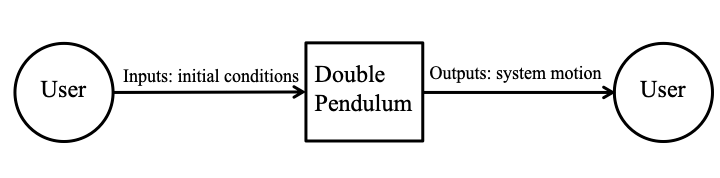
Fig:sysCtxDiag shows the system context. A circle represents an entity external to the software, the user in this case. A rectangle represents the software system itself (DblPend). Arrows are used to show the data flow between the system and its environment.

System Context
System Context

The interaction between the product and the user is through an application programming interface. The responsibilities of the user and the system are as follows:

  • User Responsibilities
    • Provide initial conditions of the physical state of the motion and the input data related to the Double Pendulum, ensuring no errors in the data entry.
    • Ensure that consistent units are used for input variables.
    • Ensure required software assumptions are appropriate for any particular problem input to the software.
  • DblPend Responsibilities
    • Detect data type mismatch, such as a string of characters input instead of a floating point number.
    • Determine if the inputs satisfy the required physical and software constraints.
    • Calculate the required outputs.
    • Generate the required graphs.

User Characteristics

The end user of DblPend should have an understanding of high school physics, high school calculus and ordinary differential equations.

System Constraints

There are no system constraints.

Specific System Description

This section first presents the problem description, which gives a high-level view of the problem to be solved. This is followed by the solution characteristics specification, which presents the assumptions, theories, and definitions that are used.

Problem Description

A system is needed to predict the motion of a double pendulum.

Terminology and Definitions

This subsection provides a list of terms that are used in the subsequent sections and their meaning, with the purpose of reducing ambiguity and making it easier to correctly understand the requirements.

  • Gravity: The force that attracts one physical body with mass to another.
  • Cartesian coordinate system: A coordinate system that specifies each point uniquely in a plane by a set of numerical coordinates, which are the signed distances to the point from two fixed perpendicular oriented lines, measured in the same unit of length (from cartesianWiki).

Physical System Description

The physical system of DblPend, as shown in Fig:dblpend, includes the following elements:

PS1: The first rod (with length of the first rod L1).

PS2: The second rod (with length of the second rod L2).

PS3: The first object.

PS4: The second object.

The physical system
The physical system

Goal Statements

Given the masses, length of the rods, initial angle of the masses and the gravitational constant, the goal statement is:

motionMass: Calculate the motion of the masses.

Solution Characteristics Specification

The instance models that govern DblPend are presented in the Instance Model Section. The information to understand the meaning of the instance models and their derivation is also presented, so that the instance models can be verified.

Assumptions

This section simplifies the original problem and helps in developing the theoretical models by filling in the missing information for the physical system. The assumptions refine the scope by providing more detail.

twoDMotion: The pendulum motion is two-dimensional (2D).

cartSys: A Cartesian coordinate system is used.

cartSysR: The Cartesian coordinate system is right-handed where positive x-axis and y-axis point right up.

yAxisDir: The direction of the y-axis is directed opposite to gravity.

startOrigin: The first rod is attached to the origin.

firstPend: The first rod has two sides. One side attaches to the origin. Another side attaches to the first object.

secondPend: The second rod has two sides. One side attaches to the first object. Another side attaches to the second object.

Theoretical Models

This section focuses on the general equations and laws that DblPend is based on.

Refname TM:acceleration
Label

Acceleration

Equation \[\symbf{a}\text{(}t\text{)}=\frac{\,d\symbf{v}\text{(}t\text{)}}{\,dt}\]
Description
  • a(t) is the acceleration (\(\frac{\text{m}}{\text{s}^{2}}\))
  • t is the time (s)
  • v(t) is the velocity (\(\frac{\text{m}}{\text{s}}\))
Source

accelerationWiki

RefBy

Refname TM:velocity
Label

Velocity

Equation \[\symbf{v}\text{(}t\text{)}=\frac{\,d\symbf{p}\text{(}t\text{)}}{\,dt}\]
Description
  • v(t) is the velocity (\(\frac{\text{m}}{\text{s}}\))
  • t is the time (s)
  • p(t) is the position (m)
Source

velocityWiki

RefBy

Refname TM:NewtonSecLawMot
Label

Newton's second law of motion

Equation \[\symbf{F}=m \symbf{a}\text{(}t\text{)}\]
Description
  • F is the force (N)
  • m is the mass (kg)
  • a(t) is the acceleration (\(\frac{\text{m}}{\text{s}^{2}}\))
Notes

The net force F on a body is proportional to the acceleration a(t) of the body, where m denotes the mass of the body as the constant of proportionality.

Source

--

RefBy

General Definitions

This section collects the laws and equations that will be used to build the instance models.

Refname GD:velocityX1
Label

The x-component of velocity of the first object

Units

\(\frac{\text{m}}{\text{s}}\)

Equation \[{v_{\text{x}1}}={w_{1}} {L_{1}} \cos\left({θ_{1}}\right)\]
Description
  • vx1 is the horizontal velocity of the first object (\(\frac{\text{m}}{\text{s}}\))
  • w1 is the angular velocity of the first object (\(\frac{\text{rad}}{\text{s}}\))
  • L1 is the length of the first rod (m)
  • θ1 is the angle of the first rod (rad)
Source

--

RefBy

Detailed derivation of the x-component of velocity:

At a given point in time, velocity is defined in DD:positionGDD

\[\symbf{v}\text{(}t\text{)}=\frac{\,d\symbf{p}\text{(}t\text{)}}{\,dt}\]

We also know the horizontal position that is defined in DD:positionXDD1

\[{p_{\text{x}1}}={L_{1}} \sin\left({θ_{1}}\right)\]

Applying this,

\[{v_{\text{x}1}}=\frac{\,d{L_{1}} \sin\left({θ_{1}}\right)}{\,dt}\]

L1 is constant with respect to time, so

\[{v_{\text{x}1}}={L_{1}} \frac{\,d\sin\left({θ_{1}}\right)}{\,dt}\]

Therefore, using the chain rule,

\[{v_{\text{x}1}}={w_{1}} {L_{1}} \cos\left({θ_{1}}\right)\]
Refname GD:velocityY1
Label

The y-component of velocity of the first object

Units

\(\frac{\text{m}}{\text{s}}\)

Equation \[{v_{\text{y}1}}={w_{1}} {L_{1}} \sin\left({θ_{1}}\right)\]
Description
  • vy1 is the vertical velocity of the first object (\(\frac{\text{m}}{\text{s}}\))
  • w1 is the angular velocity of the first object (\(\frac{\text{rad}}{\text{s}}\))
  • L1 is the length of the first rod (m)
  • θ1 is the angle of the first rod (rad)
Source

--

RefBy

Detailed derivation of the y-component of velocity:

At a given point in time, velocity is defined in DD:positionGDD

\[\symbf{v}\text{(}t\text{)}=\frac{\,d\symbf{p}\text{(}t\text{)}}{\,dt}\]

We also know the vertical position that is defined in DD:positionYDD1

\[{p_{\text{y}1}}=-{L_{1}} \cos\left({θ_{1}}\right)\]

Applying this,

\[{v_{\text{y}1}}=-\left(\frac{\,d{L_{1}} \cos\left({θ_{1}}\right)}{\,dt}\right)\]

L1 is constant with respect to time, so

\[{v_{\text{y}1}}=-{L_{1}} \frac{\,d\cos\left({θ_{1}}\right)}{\,dt}\]

Therefore, using the chain rule,

\[{v_{\text{y}1}}={w_{1}} {L_{1}} \sin\left({θ_{1}}\right)\]
Refname GD:velocityX2
Label

The x-component of velocity of the second object

Units

\(\frac{\text{m}}{\text{s}}\)

Equation \[{v_{\text{x}2}}={v_{\text{x}1}}+{w_{2}} {L_{2}} \cos\left({θ_{2}}\right)\]
Description
  • vx2 is the horizontal velocity of the second object (\(\frac{\text{m}}{\text{s}}\))
  • vx1 is the horizontal velocity of the first object (\(\frac{\text{m}}{\text{s}}\))
  • w2 is the angular velocity of the second object (\(\frac{\text{rad}}{\text{s}}\))
  • L2 is the length of the second rod (m)
  • θ2 is the angle of the second rod (rad)
Source

--

RefBy

Detailed derivation of the x-component of velocity:

At a given point in time, velocity is defined in DD:positionGDD

\[\symbf{v}\text{(}t\text{)}=\frac{\,d\symbf{p}\text{(}t\text{)}}{\,dt}\]

We also know the horizontal position that is defined in DD:positionXDD2

\[{p_{\text{x}2}}={p_{\text{x}1}}+{L_{2}} \sin\left({θ_{2}}\right)\]

Applying this,

\[{v_{\text{x}2}}=\frac{\,d{p_{\text{x}1}}+{L_{2}} \sin\left({θ_{2}}\right)}{\,dt}\]

L1 is constant with respect to time, so

\[{v_{\text{x}2}}={v_{\text{x}1}}+{w_{2}} {L_{2}} \cos\left({θ_{2}}\right)\]
Refname GD:velocityY2
Label

The y-component of velocity of the second object

Units

\(\frac{\text{m}}{\text{s}}\)

Equation \[{v_{\text{y}2}}={v_{\text{y}1}}+{w_{2}} {L_{2}} \sin\left({θ_{2}}\right)\]
Description
  • vy2 is the vertical velocity of the second object (\(\frac{\text{m}}{\text{s}}\))
  • vy1 is the vertical velocity of the first object (\(\frac{\text{m}}{\text{s}}\))
  • w2 is the angular velocity of the second object (\(\frac{\text{rad}}{\text{s}}\))
  • L2 is the length of the second rod (m)
  • θ2 is the angle of the second rod (rad)
Source

--

RefBy

Detailed derivation of the y-component of velocity:

At a given point in time, velocity is defined in DD:positionGDD

\[\symbf{v}\text{(}t\text{)}=\frac{\,d\symbf{p}\text{(}t\text{)}}{\,dt}\]

We also know the vertical position that is defined in DD:positionYDD2

\[{p_{\text{y}2}}={p_{\text{y}1}}-{L_{2}} \cos\left({θ_{2}}\right)\]

Applying this,

\[{v_{\text{y}2}}=-\left(\frac{\,d{p_{\text{y}1}}-{L_{2}} \cos\left({θ_{2}}\right)}{\,dt}\right)\]

Therefore, using the chain rule,

\[{v_{\text{y}2}}={v_{\text{y}1}}+{w_{2}} {L_{2}} \sin\left({θ_{2}}\right)\]
Refname GD:accelerationX1
Label

The x-component of acceleration of the first object

Units

\(\frac{\text{m}}{\text{s}^{2}}\)

Equation \[{a_{\text{x}1}}=-{w_{1}}^{2} {L_{1}} \sin\left({θ_{1}}\right)+{α_{1}} {L_{1}} \cos\left({θ_{1}}\right)\]
Description
  • ax1 is the horizontal acceleration of the first object (\(\frac{\text{m}}{\text{s}^{2}}\))
  • w1 is the angular velocity of the first object (\(\frac{\text{rad}}{\text{s}}\))
  • L1 is the length of the first rod (m)
  • θ1 is the angle of the first rod (rad)
  • α1 is the angular acceleration of the first object (\(\frac{\text{rad}}{\text{s}^{2}}\))
Source

--

RefBy

IM:calOfAngle2

Detailed derivation of the x-component of acceleration:

Our acceleration is:

\[\symbf{a}\text{(}t\text{)}=\frac{\,d\symbf{v}\text{(}t\text{)}}{\,dt}\]

Earlier, we found the horizontal velocity to be

\[{v_{\text{x}1}}={w_{1}} {L_{1}} \cos\left({θ_{1}}\right)\]

Applying this to our equation for acceleration

\[{a_{\text{x}1}}=\frac{\,d{w_{1}} {L_{1}} \cos\left({θ_{1}}\right)}{\,dt}\]

By the product and chain rules, we find

\[{a_{\text{x}1}}=\frac{\,d{w_{1}}}{\,dt} {L_{1}} \cos\left({θ_{1}}\right)-{w_{1}} {L_{1}} \sin\left({θ_{1}}\right) \frac{\,d{θ_{1}}}{\,dt}\]

Simplifying,

\[{a_{\text{x}1}}=-{w_{1}}^{2} {L_{1}} \sin\left({θ_{1}}\right)+{α_{1}} {L_{1}} \cos\left({θ_{1}}\right)\]
Refname GD:accelerationY1
Label

The y-component of acceleration of the first object

Units

\(\frac{\text{m}}{\text{s}^{2}}\)

Equation \[{a_{\text{y}1}}={w_{1}}^{2} {L_{1}} \cos\left({θ_{1}}\right)+{α_{1}} {L_{1}} \sin\left({θ_{1}}\right)\]
Description
  • ay1 is the vertical acceleration of the first object (\(\frac{\text{m}}{\text{s}^{2}}\))
  • w1 is the angular velocity of the first object (\(\frac{\text{rad}}{\text{s}}\))
  • L1 is the length of the first rod (m)
  • θ1 is the angle of the first rod (rad)
  • α1 is the angular acceleration of the first object (\(\frac{\text{rad}}{\text{s}^{2}}\))
Source

--

RefBy

IM:calOfAngle2

Detailed derivation of the y-component of acceleration:

Our acceleration is:

\[\symbf{a}\text{(}t\text{)}=\frac{\,d\symbf{v}\text{(}t\text{)}}{\,dt}\]

Earlier, we found the vertical velocity to be

\[{v_{\text{y}1}}={w_{1}} {L_{1}} \sin\left({θ_{1}}\right)\]

Applying this to our equation for acceleration

\[{a_{\text{y}1}}=\frac{\,d{w_{1}} {L_{1}} \sin\left({θ_{1}}\right)}{\,dt}\]

By the product and chain rules, we find

\[{a_{\text{y}1}}=\frac{\,d{w_{1}}}{\,dt} {L_{1}} \sin\left({θ_{1}}\right)+{w_{1}} {L_{1}} \cos\left({θ_{1}}\right) \frac{\,d{θ_{1}}}{\,dt}\]

Simplifying,

\[{a_{\text{y}1}}={w_{1}}^{2} {L_{1}} \cos\left({θ_{1}}\right)+{α_{1}} {L_{1}} \sin\left({θ_{1}}\right)\]
Refname GD:accelerationX2
Label

The x-component of acceleration of the second object

Units

\(\frac{\text{m}}{\text{s}^{2}}\)

Equation \[{a_{\text{x}2}}={a_{\text{x}1}}-{w_{2}}^{2} {L_{2}} \sin\left({θ_{2}}\right)+{α_{2}} {L_{2}} \cos\left({θ_{2}}\right)\]
Description
  • ax2 is the horizontal acceleration of the second object (\(\frac{\text{m}}{\text{s}^{2}}\))
  • ax1 is the horizontal acceleration of the first object (\(\frac{\text{m}}{\text{s}^{2}}\))
  • w2 is the angular velocity of the second object (\(\frac{\text{rad}}{\text{s}}\))
  • L2 is the length of the second rod (m)
  • θ2 is the angle of the second rod (rad)
  • α2 is the angular acceleration of the second object (\(\frac{\text{rad}}{\text{s}^{2}}\))
Source

--

RefBy

IM:calOfAngle2

Detailed derivation of the x-component of acceleration:

Our acceleration is:

\[\symbf{a}\text{(}t\text{)}=\frac{\,d\symbf{v}\text{(}t\text{)}}{\,dt}\]

Earlier, we found the horizontal velocity to be

\[{v_{\text{x}2}}={v_{\text{x}1}}+{w_{2}} {L_{2}} \cos\left({θ_{2}}\right)\]

Applying this to our equation for acceleration

\[{a_{\text{x}2}}=\frac{\,d{v_{\text{x}1}}+{w_{2}} {L_{2}} \cos\left({θ_{2}}\right)}{\,dt}\]

By the product and chain rules, we find

\[{a_{\text{x}2}}={a_{\text{x}1}}-{w_{2}}^{2} {L_{2}} \sin\left({θ_{2}}\right)+{α_{2}} {L_{2}} \cos\left({θ_{2}}\right)\]
Refname GD:accelerationY2
Label

The y-component of acceleration of the second object

Units

\(\frac{\text{m}}{\text{s}^{2}}\)

Equation \[{a_{\text{y}2}}={a_{\text{y}1}}+{w_{2}}^{2} {L_{2}} \cos\left({θ_{2}}\right)+{α_{2}} {L_{2}} \sin\left({θ_{2}}\right)\]
Description
  • ay2 is the vertical acceleration of the second object (\(\frac{\text{m}}{\text{s}^{2}}\))
  • ay1 is the vertical acceleration of the first object (\(\frac{\text{m}}{\text{s}^{2}}\))
  • w2 is the angular velocity of the second object (\(\frac{\text{rad}}{\text{s}}\))
  • L2 is the length of the second rod (m)
  • θ2 is the angle of the second rod (rad)
  • α2 is the angular acceleration of the second object (\(\frac{\text{rad}}{\text{s}^{2}}\))
Source

--

RefBy

IM:calOfAngle2

Detailed derivation of the y-component of acceleration:

Our acceleration is:

\[\symbf{a}\text{(}t\text{)}=\frac{\,d\symbf{v}\text{(}t\text{)}}{\,dt}\]

Earlier, we found the horizontal velocity to be

\[{v_{\text{y}2}}={v_{\text{y}1}}+{w_{2}} {L_{2}} \sin\left({θ_{2}}\right)\]

Applying this to our equation for acceleration

\[{a_{\text{y}2}}=\frac{\,d{v_{\text{y}1}}+{w_{2}} {L_{2}} \sin\left({θ_{2}}\right)}{\,dt}\]

By the product and chain rules, we find

\[{a_{\text{y}2}}={a_{\text{y}1}}+{w_{2}}^{2} {L_{2}} \cos\left({θ_{2}}\right)+{α_{2}} {L_{2}} \sin\left({θ_{2}}\right)\]
Refname GD:xForce1
Label

Horizontal force on the first object

Units

N

Equation \[\symbf{F}=m \symbf{a}\text{(}t\text{)}=-{\symbf{T}_{1}} \sin\left({θ_{1}}\right)+{\symbf{T}_{2}} \sin\left({θ_{2}}\right)\]
Description
  • F is the force (N)
  • m is the mass (kg)
  • a(t) is the acceleration (\(\frac{\text{m}}{\text{s}^{2}}\))
  • T1 is the tension of the first object (N)
  • θ1 is the angle of the first rod (rad)
  • T2 is the tension of the second object (N)
  • θ2 is the angle of the second rod (rad)
Source

--

RefBy

IM:calOfAngle2

Detailed derivation of force on the first object:

\[\symbf{F}=m \symbf{a}\text{(}t\text{)}=-{\symbf{T}_{1}} \sin\left({θ_{1}}\right)+{\symbf{T}_{2}} \sin\left({θ_{2}}\right)\]
Refname GD:yForce1
Label

Vertical force on the first object

Units

N

Equation \[\symbf{F}=m \symbf{a}\text{(}t\text{)}={\symbf{T}_{1}} \cos\left({θ_{1}}\right)-{\symbf{T}_{2}} \cos\left({θ_{2}}\right)-{m_{1}} \symbf{g}\]
Description
  • F is the force (N)
  • m is the mass (kg)
  • a(t) is the acceleration (\(\frac{\text{m}}{\text{s}^{2}}\))
  • T1 is the tension of the first object (N)
  • θ1 is the angle of the first rod (rad)
  • T2 is the tension of the second object (N)
  • θ2 is the angle of the second rod (rad)
  • m1 is the mass of the first object (kg)
  • g is the gravitational acceleration (\(\frac{\text{m}}{\text{s}^{2}}\))
Source

--

RefBy

IM:calOfAngle2

Detailed derivation of force on the first object:

\[\symbf{F}=m \symbf{a}\text{(}t\text{)}={\symbf{T}_{1}} \cos\left({θ_{1}}\right)-{\symbf{T}_{2}} \cos\left({θ_{2}}\right)-{m_{1}} \symbf{g}\]
Refname GD:xForce2
Label

Horizontal force on the second object

Units

N

Equation \[\symbf{F}=m \symbf{a}\text{(}t\text{)}=-{\symbf{T}_{2}} \sin\left({θ_{2}}\right)\]
Description
  • F is the force (N)
  • m is the mass (kg)
  • a(t) is the acceleration (\(\frac{\text{m}}{\text{s}^{2}}\))
  • T2 is the tension of the second object (N)
  • θ2 is the angle of the second rod (rad)
Source

--

RefBy

IM:calOfAngle2

Detailed derivation of force on the second object:

\[\symbf{F}=m \symbf{a}\text{(}t\text{)}=-{\symbf{T}_{2}} \sin\left({θ_{2}}\right)\]
Refname GD:yForce2
Label

Vertical force on the second object

Units

N

Equation \[\symbf{F}=m \symbf{a}\text{(}t\text{)}={\symbf{T}_{2}} \cos\left({θ_{2}}\right)-{m_{2}} \symbf{g}\]
Description
  • F is the force (N)
  • m is the mass (kg)
  • a(t) is the acceleration (\(\frac{\text{m}}{\text{s}^{2}}\))
  • T2 is the tension of the second object (N)
  • θ2 is the angle of the second rod (rad)
  • m2 is the mass of the second object (kg)
  • g is the gravitational acceleration (\(\frac{\text{m}}{\text{s}^{2}}\))
Source

--

RefBy

IM:calOfAngle2

Detailed derivation of force on the second object:

\[\symbf{F}=m \symbf{a}\text{(}t\text{)}={\symbf{T}_{2}} \cos\left({θ_{2}}\right)-{m_{2}} \symbf{g}\]

Data Definitions

This section collects and defines all the data needed to build the instance models.

Refname DD:positionGDD
Label

Velocity

Symbol

v(t)

Units

\(\frac{\text{m}}{\text{s}}\)

Equation \[\symbf{v}\text{(}t\text{)}=\frac{\,d\symbf{p}\text{(}t\text{)}}{\,dt}\]
Description
  • v(t) is the velocity (\(\frac{\text{m}}{\text{s}}\))
  • t is the time (s)
  • p(t) is the position (m)
Source

--

RefBy

GD:velocityY2, GD:velocityY1, GD:velocityX2, and GD:velocityX1

Refname DD:positionXDD1
Label

Horizontal position of the first object

Symbol

px1

Units

m

Equation \[{p_{\text{x}1}}={L_{1}} \sin\left({θ_{1}}\right)\]
Description
  • px1 is the horizontal position of the first object (m)
  • L1 is the length of the first rod (m)
  • θ1 is the angle of the first rod (rad)
Notes

px1 is the horizontal position

px1 is shown in Fig:dblpend.

Source

--

RefBy

GD:velocityX1

Refname DD:positionYDD1
Label

Vertical position of the first object

Symbol

py1

Units

m

Equation \[{p_{\text{y}1}}=-{L_{1}} \cos\left({θ_{1}}\right)\]
Description
  • py1 is the vertical position of the first object (m)
  • L1 is the length of the first rod (m)
  • θ1 is the angle of the first rod (rad)
Notes

py1 is the vertical position

py1 is shown in Fig:dblpend.

Source

--

RefBy

GD:velocityY1

Refname DD:positionXDD2
Label

Horizontal position of the second object

Symbol

px2

Units

m

Equation \[{p_{\text{x}2}}={p_{\text{x}1}}+{L_{2}} \sin\left({θ_{2}}\right)\]
Description
  • px2 is the horizontal position of the second object (m)
  • px1 is the horizontal position of the first object (m)
  • L2 is the length of the second rod (m)
  • θ2 is the angle of the second rod (rad)
Notes

px2 is the horizontal position

px2 is shown in Fig:dblpend.

Source

--

RefBy

GD:velocityX2

Refname DD:positionYDD2
Label

Vertical position of the second object

Symbol

py2

Units

m

Equation \[{p_{\text{y}2}}={p_{\text{y}1}}-{L_{2}} \cos\left({θ_{2}}\right)\]
Description
  • py2 is the vertical position of the second object (m)
  • py1 is the vertical position of the first object (m)
  • L2 is the length of the second rod (m)
  • θ2 is the angle of the second rod (rad)
Notes

py2 is the vertical position

py2 is shown in Fig:dblpend.

Source

--

RefBy

GD:velocityY2

Refname DD:accelerationGDD
Label

Acceleration

Symbol

a(t)

Units

\(\frac{\text{m}}{\text{s}^{2}}\)

Equation \[\symbf{a}\text{(}t\text{)}=\frac{\,d\symbf{v}\text{(}t\text{)}}{\,dt}\]
Description
  • a(t) is the acceleration (\(\frac{\text{m}}{\text{s}^{2}}\))
  • t is the time (s)
  • v(t) is the velocity (\(\frac{\text{m}}{\text{s}}\))
Source

--

RefBy

Refname DD:forceGDD
Label

Force

Symbol

F

Units

N

Equation \[\symbf{F}=m \symbf{a}\text{(}t\text{)}\]
Description
  • F is the force (N)
  • m is the mass (kg)
  • a(t) is the acceleration (\(\frac{\text{m}}{\text{s}^{2}}\))
Source

--

RefBy

Instance Models

This section transforms the problem defined in the problem description into one which is expressed in mathematical terms. It uses concrete symbols defined in the data definitions to replace the abstract symbols in the models identified in theoretical models and general definitions.

Refname IM:calOfAngle1
Label

Calculation of angle of first rod

Input

L1, L2, m1, m2, θ1, θ2

Output

θ1

Input Constraints \[{L_{1}}\gt{}0\] \[{L_{2}}\gt{}0\] \[{m_{1}}\gt{}0\] \[{m_{2}}\gt{}0\]
Output Constraints
Equation \[{α_{1}}\left({θ_{1}},{θ_{2}},{w_{1}},{w_{2}}\right)=\frac{-g \left(2 {m_{1}}+{m_{2}}\right) \sin\left({θ_{1}}\right)-{m_{2}} g \sin\left({θ_{1}}-2 {θ_{2}}\right)-2 \sin\left({θ_{1}}-{θ_{2}}\right) {m_{2}} \left({w_{2}}^{2} {L_{2}}+{w_{1}}^{2} {L_{1}} \cos\left({θ_{1}}-{θ_{2}}\right)\right)}{{L_{1}} \left(2 {m_{1}}+{m_{2}}-{m_{2}} \cos\left(2 {θ_{1}}-2 {θ_{2}}\right)\right)}\]
Description
  • α1 is the angular acceleration of the first object (\(\frac{\text{rad}}{\text{s}^{2}}\))
  • θ1 is the angle of the first rod (rad)
  • θ2 is the angle of the second rod (rad)
  • w1 is the angular velocity of the first object (\(\frac{\text{rad}}{\text{s}}\))
  • w2 is the angular velocity of the second object (\(\frac{\text{rad}}{\text{s}}\))
  • g is the magnitude of gravitational acceleration (\(\frac{\text{m}}{\text{s}^{2}}\))
  • m1 is the mass of the first object (kg)
  • m2 is the mass of the second object (kg)
  • L2 is the length of the second rod (m)
  • L1 is the length of the first rod (m)
Notes

θ1 is calculated by solving the ODE here together with the initial conditions and IM:calOfAngle2.

Source

--

RefBy

FR:Output-Values, FR:Calculate-Angle-Of-Rod, and IM:calOfAngle2

Refname IM:calOfAngle2
Label

Calculation of angle of second rod

Input

L1, L2, m1, m2, θ1, θ2

Output

θ2

Input Constraints \[{L_{1}}\gt{}0\] \[{L_{2}}\gt{}0\] \[{m_{1}}\gt{}0\] \[{m_{2}}\gt{}0\]
Output Constraints
Equation \[{α_{2}}\left({θ_{1}},{θ_{2}},{w_{1}},{w_{2}}\right)=\frac{2 \sin\left({θ_{1}}-{θ_{2}}\right) \left({w_{1}}^{2} {L_{1}} \left({m_{1}}+{m_{2}}\right)+g \left({m_{1}}+{m_{2}}\right) \cos\left({θ_{1}}\right)+{w_{2}}^{2} {L_{2}} {m_{2}} \cos\left({θ_{1}}-{θ_{2}}\right)\right)}{{L_{2}} \left(2 {m_{1}}+{m_{2}}-{m_{2}} \cos\left(2 {θ_{1}}-2 {θ_{2}}\right)\right)}\]
Description
  • α2 is the angular acceleration of the second object (\(\frac{\text{rad}}{\text{s}^{2}}\))
  • θ1 is the angle of the first rod (rad)
  • θ2 is the angle of the second rod (rad)
  • w1 is the angular velocity of the first object (\(\frac{\text{rad}}{\text{s}}\))
  • w2 is the angular velocity of the second object (\(\frac{\text{rad}}{\text{s}}\))
  • L1 is the length of the first rod (m)
  • m1 is the mass of the first object (kg)
  • m2 is the mass of the second object (kg)
  • g is the magnitude of gravitational acceleration (\(\frac{\text{m}}{\text{s}^{2}}\))
  • L2 is the length of the second rod (m)
Notes

θ2 is calculated by solving the ODE here together with the initial conditions and IM:calOfAngle1.

Source

--

RefBy

FR:Output-Values, FR:Calculate-Angle-Of-Rod, IM:calOfAngle2, and IM:calOfAngle1

Detailed derivation of angle of the second rod:

By solving equations GD:xForce2 and GD:yForce2 for T2 sin(θ2) and T2 cos(θ2) and then substituting into equation GD:xForce1 and GD:yForce1 , We can get equations 1 and 2:

\[{m_{1}} {a_{\text{x}1}}=-{\symbf{T}_{1}} \sin\left({θ_{1}}\right)-{m_{2}} {a_{\text{x}2}}\]

\[{m_{1}} {a_{\text{y}1}}={\symbf{T}_{1}} \cos\left({θ_{1}}\right)-{m_{2}} {a_{\text{y}2}}-{m_{2}} g-{m_{1}} g\]

Multiply the equation 1 by cos(θ1) and the equation 2 by sin(θ1) and rearrange to get:

\[{\symbf{T}_{1}} \sin\left({θ_{1}}\right) \cos\left({θ_{1}}\right)=-\cos\left({θ_{1}}\right) \left({m_{1}} {a_{\text{x}1}}+{m_{2}} {a_{\text{x}2}}\right)\]

\[{\symbf{T}_{1}} \sin\left({θ_{1}}\right) \cos\left({θ_{1}}\right)=\sin\left({θ_{1}}\right) \left({m_{1}} {a_{\text{y}1}}+{m_{2}} {a_{\text{y}2}}+{m_{2}} g+{m_{1}} g\right)\]

This leads to the equation 3

\[\sin\left({θ_{1}}\right) \left({m_{1}} {a_{\text{y}1}}+{m_{2}} {a_{\text{y}2}}+{m_{2}} g+{m_{1}} g\right)=-\cos\left({θ_{1}}\right) \left({m_{1}} {a_{\text{x}1}}+{m_{2}} {a_{\text{x}2}}\right)\]

Next, multiply equation GD:xForce2 by cos(θ2) and equation GD:yForce2 by sin(θ2) and rearrange to get:

\[{\symbf{T}_{2}} \sin\left({θ_{2}}\right) \cos\left({θ_{2}}\right)=-\cos\left({θ_{2}}\right) {m_{2}} {a_{\text{x}2}}\]

\[{\symbf{T}_{1}} \sin\left({θ_{2}}\right) \cos\left({θ_{2}}\right)=\sin\left({θ_{2}}\right) \left({m_{2}} {a_{\text{y}2}}+{m_{2}} g\right)\]

which leads to equation 4

\[\sin\left({θ_{2}}\right) \left({m_{2}} {a_{\text{y}2}}+{m_{2}} g\right)=-\cos\left({θ_{2}}\right) {m_{2}} {a_{\text{x}2}}\]

By giving equations GD:accelerationX1 and GD:accelerationX2 and GD:accelerationY1 and GD:accelerationY2 plus additional two equations, 3 and 4, we can get IM:calOfAngle1 and IM:calOfAngle2 via a computer algebra program:

Data Constraints

The Data Constraints Table shows the data constraints on the input variables. The column for physical constraints gives the physical limitations on the range of values that can be taken by the variable. The uncertainty column provides an estimate of the confidence with which the physical quantities can be measured. This information would be part of the input if one were performing an uncertainty quantification exercise. The constraints are conservative to give the user of the model the flexibility to experiment with unusual situations. The column of typical values is intended to provide a feel for a common scenario.

Var Physical Constraints Typical Value Uncert.
L1 L1 > 0 1.0 m 10%
L2 L2 > 0 1.0 m 10%
m1 m1 > 0 0.5 kg 10%
m2 m2 > 0 0.5 kg 10%

Input Data Constraints

Properties of a Correct Solution

The Data Constraints Table shows the data constraints on the output variables. The column for physical constraints gives the physical limitations on the range of values that can be taken by the variable.

Var Physical Constraints
θ1 θ1 > 0
θ2 θ2 > 0

Output Data Constraints

Requirements

This section provides the functional requirements, the tasks and behaviours that the software is expected to complete, and the non-functional requirements, the qualities that the software is expected to exhibit.

Functional Requirements

This section provides the functional requirements, the tasks and behaviours that the software is expected to complete.

Input-Values: Input the values from Tab:ReqInputs.

Verify-Input-Values: Check the entered input values to ensure that they do not exceed the data constraints. If any of the input values are out of bounds, an error message is displayed and the calculations stop.

Calculate-Angle-Of-Rod: Calculate the following values: θ1 and θ2 (from IM:calOfAngle1 and IM:calOfAngle2).

Output-Values: Output θ1 and θ2 (from IM:calOfAngle1 and IM:calOfAngle2).

Symbol Description Units
L1 Length of the first rod m
L2 Length of the second rod m
m1 Mass of the first object kg
m2 Mass of the second object kg

Required Inputs following FR:Input-Values

Non-Functional Requirements

This section provides the non-functional requirements, the qualities that the software is expected to exhibit.

Correct: The outputs of the code have the properties of a correct solution.

Portable: The code is able to be run in different environments.

Traceability Matrices and Graphs

The purpose of the traceability matrices is to provide easy references on what has to be additionally modified if a certain component is changed. Every time a component is changed, the items in the column of that component that are marked with an "X" should be modified as well. Tab:TraceMatAvsA shows the dependencies of the assumptions on each other. Tab:TraceMatAvsAll shows the dependencies of the data definitions, theoretical models, general definitions, instance models, requirements, likely changes, and unlikely changes on the assumptions. Tab:TraceMatRefvsRef shows the dependencies of the data definitions, theoretical models, general definitions, and instance models on each other. Tab:TraceMatAllvsR shows the dependencies of the requirements and goal statements on the data definitions, theoretical models, general definitions, and instance models.

The purpose of the traceability graphs is also to provide easy references on what has to be additionally modified if a certain component is changed. The arrows in the graphs represent dependencies. The component at the tail of an arrow is depended on by the component at the head of that arrow. Therefore, if a component is changed, the components that it points to should also be changed. Fig:TraceGraphAvsA shows the dependencies of assumptions on each other. Fig:TraceGraphAvsAll shows the dependencies of data definitions, theoretical models, general definitions, instance models, requirements, likely changes, and unlikely changes on the assumptions. Fig:TraceGraphRefvsRef shows the dependencies of data definitions, theoretical models, general definitions, and instance models on each other. Fig:TraceGraphAllvsR shows the dependencies of requirements and goal statements on the data definitions, theoretical models, general definitions, and instance models. Fig:TraceGraphAllvsAll shows the dependencies of dependencies of assumptions, models, definitions, requirements, goals, and changes with each other.

TraceGraphAvsA
TraceGraphAvsA
TraceGraphAvsAll
TraceGraphAvsAll
TraceGraphRefvsRef
TraceGraphRefvsRef
TraceGraphAllvsR
TraceGraphAllvsR
TraceGraphAllvsAll
TraceGraphAllvsAll

For convenience, the following graphs can be found at the links below:

Values of Auxiliary Constants

There are no auxiliary constants.

References